Swimmer simulation using robot manipulator dynamics under steady water

doi:10.4236/ns.2010.29117

Paper Menu >>

Journal Menu >>

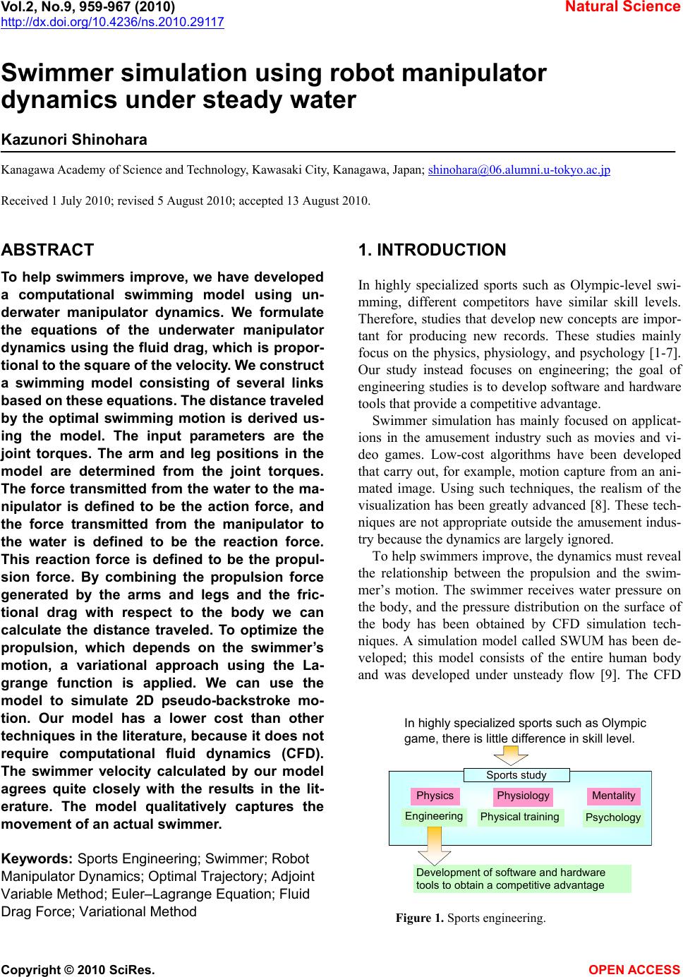Vol.2, No.9, 959-967 (2010) Natural Science

http://dx.doi.org/10.4236/ns.2010.29117

Swimmer simulation using robot manipulator

dynamics under steady water

Kazunori Shinohara

Kanagawa Academy of Science and Technology, Kawasaki City, Kanagawa, Japan; [email protected]

Received 1 July 2010; revised 5 August 2010; accepted 13 August 2010.

ABSTRACT

To help swimmers improve, we have developed

a computational swimming model using un-

derwater manipulator dynamics. We formulate

the equations of the underwater manipulator

dynamics using the fluid drag, which is propor-

tional to the square of the velocity. We construct

a swimming model consisting of several links

based on these equations. The distance traveled

by the optimal swimming motion is derived us-

ing the model. The input parameters are the

joint torques. The arm and leg positions in the

model are determined from the joint torques.

The force transmitted from the water to the ma-

nipulator is defined to be the action force, and

the force transmitted from the manipulator to

the water is defined to be the reaction force.

This reaction force is defined to be the propul-

sion force. By combining the propulsion force

generated by the arms and legs and the fric-

tional drag with respect to the body we can

calculate the distance traveled. To optimize the

propulsion, which depends on the swimmer’s

motion, a variational approach using the La-

grange function is applied. We can use the

model to simulate 2D pseudo-backstroke mo-

tion. Our model has a lower cost than other

techniques in the literature, because it does not

require computational fluid dynamics (CFD).

The swimmer velocity calculated by our model

agrees quite closely with the results in the lit-

erature. The model qualitatively captures the

movement of an actual swimmer.

Keywords: Sports Engineering; Swimmer; Robot

Manipulator Dynamics; Optimal Trajectory; Adjoint

Variable Method; Euler–Lagrange Equation; Fluid

Drag Force; Variational Method

1. INTRODUCTION

In highly specialized sports such as Olympic-level swi-

mming, different competitors have similar skill levels.

Therefore, studies that develop new concepts are impor-

tant for producing new records. These studies mainly

focus on the physics, physiology, and psychology [1-7].

Our study instead focuses on engineering; the goal of

engineering studies is to develop software and hardware

tools that provide a competitive advantage.

Swimmer simulation has mainly focused on applicat-

ions in the amusement industry such as movies and vi-

deo games. Low-cost algorithms have been developed

that carry out, for example, motion capture from an ani-

mated image. Using such techniques, the realism of the

visualization has been greatly advanced [8]. These tech-

niques are not appropriate outside the amusement indus-

try because the dynamics are largely ignored.

To help swimmers improve, the dynamics must reveal

the relationship between the propulsion and the swim-

mer’s motion. The swimmer receives water pressure on

the body, and the pressure distribution on the surface of

the body has been obtained by CFD simulation tech-

niques. A simulation model called SWUM has been de-

veloped; this model consists of the entire human body

and was developed under unsteady flow [9]. The CFD

Development of software and hardware

tools to obtain a competitive advantage

In highly specialized sports such as Olympic

game, there is little difference in skill level.

Physiology Mentality

Physics

Physical training Psychology

Engineering

Sports study

Figure 1. Sports engineering.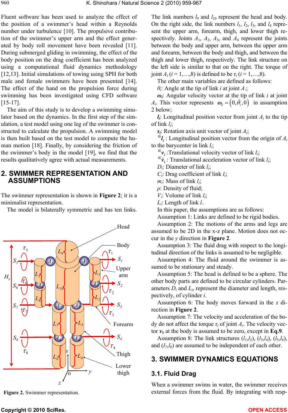

K. Shinohara / Natural Science 2 (2010) 959-967

960

Fluent software has been used to analyze the effect of

the position of a swimmer’s head within a Reynolds

number under turbulence [10]. The propulsive contribu-

tion of the swimmer’s upper arm and the effect gener-

ated by body roll movement have been revealed [11].

During submerged gliding in swimming, the effect of the

body position on the drag coefficient has been analyzed

using a computational fluid dynamics methodology

[12,13]. Initial simulations of towing using SPH for both

male and female swimmers have been presented [14].

The effect of the hand on the propulsion force during

swimming has been investigated using CFD software

[15-17].

The aim of this study is to develop a swimming simu-

lator based on the dynamics. In the first step of the sim-

ulation, a test model using one leg of the swimmer is con-

structed to calculate the propulsion. A swimming model

is then built based on the test model to compute the hu-

man motion [18]. Finally, by considering the friction of

the swimmer’s body in the model [19], we find that the

results qualitatively agree with actual measurements.

2. SWIMMER REPRESENTATION AND

ASSUMPTIONS

The swimmer representation is shown in Figure 2; it is a

minimalist representation.

The model is bilaterally symmetric and has ten links.

Head

Body

Upper

arm

Forearm

Lower

thigh

Thigh



Figure 2. Swimmer representation.

The link numbers l9 and l10 represent the head and body.

On the right side, the link numbers l1, l2, l3, and l4 repre-

sent the upper arm, forearm, thigh, and lower thigh re-

spectively. Joints A1, A2, A3, and A4 represent the joints

between the body and upper arm, between the upper arm

and forearm, between the body and thigh, and between the

thigh and lower thigh, respectively. The link structure on

the left side is similar to that on the right. The torque of

joint Ai (i = 1,…,8) is defined to be τi (i = 1,…,8).

The other main variables are defined as follows:

θi: Angle at the tip of link i at joint A

;

ωi: Angular velocity vector at the tip of link i at joint

Ai. This vector represents



0,, 0





ω in assumption

2 below;

li: Longitudinal position vector from joint Ai to the tip

of link li;

si: Rotation axis unit vector of joint Ai;

l: Longitudinal position vector from the origin of Ai

to the barycenter in link li;

v:Translational velocity vector of link li;



v: Translational acceleration vector of link li;

Di: Diameter of link li;

Ci: Drag coefficient of link li;

mi: Mass of link li;

ρ: Density of fluid;

Vi: Volume of link li;

Li: Length of link l

i。

In this paper, the assumptions are as follows:

Assumption 1: Links are defined to be rigid bodies.

Assumption 2: The motions of the arms and legs are

assumed to be 2D in the x-z plane. Motion does not oc-

cur in the y direction in Figure 2.

Assumption 3: The fluid drag with respect to the longi-

tudinal direction of the links is assumed to be negligible.

Assumption 4: The fluid around the swimmer is as-

sumed to be stationary and steady.

Assumption 5: The head is defined to be a sphere. The

other body parts are defined to be circular cylinders. Par-

ameters Di and Li, represent the diameter and length, res-

pectively, of cylinder i.

Assumption 6: The body moves forward in the x di-

rection in Figure 2.

Assumption 7: The velocity and acceleration of the bo-

dy do not affect the torque τi of joint Ai. The velocity vec-

tor v0 at the body is assumed to be zero, except in Eq.9.

Assumption 8: The link structures (l1,l2), (l3,l4), (l5,l6),

and (l7,l8) are assumed to be independent of each other.

3. SWIMMER DYNAMICS EQUATIONS

3.1. Fluid Drag

When a swimmer swims in water, the swimmer receives

external forces from the fluid. By integrating with resp-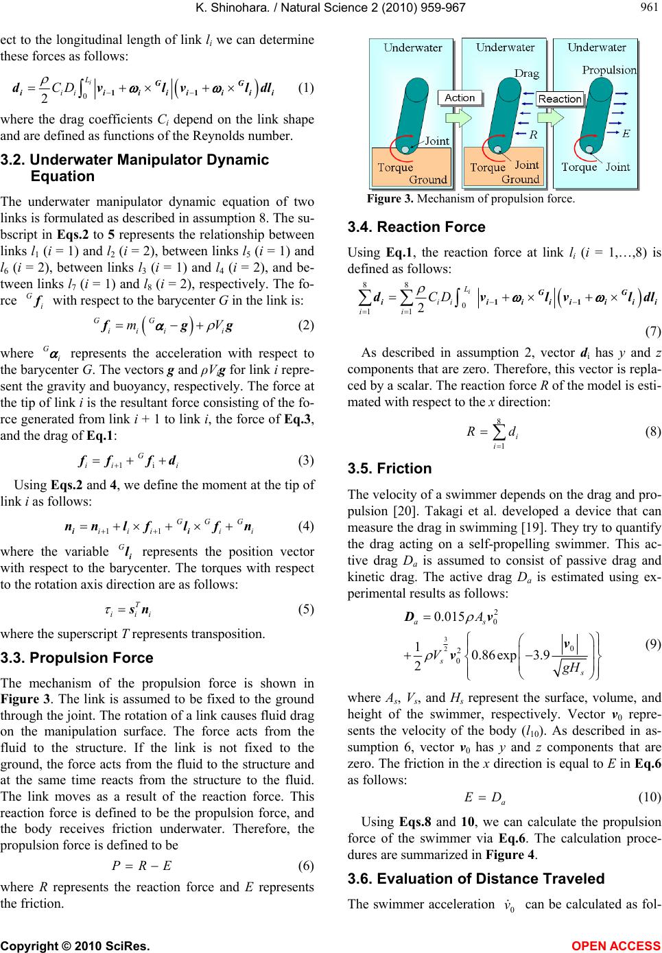

K. Shinohara. / Natural Science 2 (2010) 959-967

961

ect to the longitudinal length of link li we can determine

these forces as follows:









11

iiiiiiii

dvlvldl



(1)

where the drag coefficients Ci depend on the link shape

and are defined as functions of the Reynolds number.

3.2. Underwater Manipulator Dynamic

Equation

The underwater manipulator dynamic equation of two

links is formulated as described in assumption 8. The su-

bscript in Eqs.2 to 5 represents the relationship between

links l1 (i = 1) and l2 (i = 2), between links l5 (i = 1) and

l6 (i = 2), between links l3 (i = 1) and l4 (i = 2), and be-

tween links l7 (i = 1) and l8 (i = 2), respectively. The fo-

rce G

f with respect to the barycenter G in the link is:



iiii





fgg



(2)

where G



represents the acceleration with respect to

the barycenter G. The vectors g and ρVig for link i repre-

sent the gravity and buoyancy, respectively. The force at

the tip of link i is the resultant force consisting of the fo-

rce generated from link i + 1 to link i, the force of Eq.3,

and the drag of Eq.1:

ii i

ff fd

(3)

Using Eqs.2 and 4, we define the moment at the tip of

link i as follows:

GG G

iiii i





nn lflfn (4)

where the variable G

l represents the position vector

with respect to the barycenter. The torques with respect

to the rotation axis direction are as follows:

iii



sn (5)

where the superscript T represents transposition.

3.3. Propulsion Force

The mechanism of the propulsion force is shown in

Figure 3. The link is assumed to be fixed to the ground

through the joint. The rotation of a link causes fluid drag

on the manipulation surface. The force acts from the

fluid to the structure. If the link is not fixed to the

ground, the force acts from the fluid to the structure and

at the same time reacts from the structure to the fluid.

The link moves as a result of the reaction force. This

reaction force is defined to be the propulsion force, and

the body receives friction underwater. Therefore, the

propulsion force is defined to be

 (6)

where R represents the reaction force and E represents

the friction.

Figure 3. Mechanism of propulsion force.

3.4. Reaction Force

Using Eq.1, the reaction force at link li (i = 1,…,8) is

defined as follows:











 11

iiiiiiii

dvlvldl



(7)

As described in assumption 2, vector di has y and z

components that are zero. Therefore, this vector is repla-

ced by a scalar. The reaction force R of the model is esti-

mated with respect to the x direction:





8

dR (8)

3.5. Friction

The velocity of a swimmer depends on the drag and pro-

pulsion [20]. Takagi et al. developed a device that can

measure the drag in swimming [19]. They try to quantify

the drag acting on a self-propelling swimmer. This ac-

tive drag Da is assumed to consist of passive drag and

kinetic drag. The active drag Da is estimated using ex-

perimental results as follows:

0.015

10.86exp 3.9

VgH





























v (9)

where As, Vs, and Hs represent the surface, volume, and

height of the swimmer, respectively. Vector v0 repre-

sents the velocity of the body (l10). As described in as-

sumption 6, vector v0 has y and z components that are

zero. The friction in the x direction is equal to E in Eq.6

as follows:



(10)

Using Eqs.8 and 10, we can calculate the propulsion

force of the swimmer via Eq.6. The calculation proce-

dures are summarized in Figure 4.

3.6. Evaluation of Distance Traveled

The swimmer acceleration 0

 can be calculated as fol-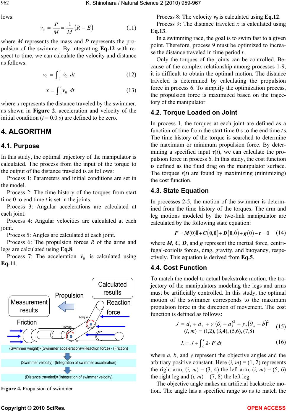

K. Shinohara / Natural Science 2 (2010) 959-967

962

lows:



v 1

 (11)

where M represents the mass and P represents the pro-

pulsion of the swimmer. By integrating Eq.12 with re-

spect to time, we can calculate the velocity and distance

as follows:

dtvv t



000  (12)

dtvx t



00 (13)

where x represents the distance traveled by the swimmer,

as shown in Figure 2. acceleration and velocity of the

initial condition (t = 0.0 s) are defined to be zero.

4. ALGORITHM

4.1. Purpose

In this study, the optimal trajectory of the manipulator is

calculated. The process from the input of the torque to

the output of the distance traveled is as follows:

Process 1: Parameters and initial conditions are set in

the model.

Process 2: The time history of the torques from start

time 0 to end time t is set in the joints.

Process 3: Angular accelerations are calculated at

each joint.

Process 4: Angular velocities are calculated at each

joint.

Process 5: Angles are calculated at each joint.

Process 6: The propulsion forces R of the arms and

legs are calculated using Eq.8.

Process 7: The acceleration 0

 is calculated using

Eq.11.

Reaction

force

(Swimmer weight)×(Swimmer acceleration)=(Reaction force) - (Friction)

Friction

Measurement

results

Calculated

results

(Swimmer velocity)=(Integration of swimmer acceleration)

(Distance traveled)=(Integration of swimmer velocity)

Torque

Propulsion

Figure 4. Propulsion of swimmer.

Process 8: The velocity v0 is calculated using Eq.12.

Process 9: The distance traveled x is calculated using

Eq.13.

In a swimming race, the goal is to swim fast to a given

point. Therefore, process 9 must be optimized to increa-

se the distance traveled in time period t.

Only the torques of the joints can be controlled. Be-

cause of the complex relationship among processes 1-9,

it is difficult to obtain the optimal motion. The distance

traveled is determined by calculating the propulsion

force in process 6. To simplify the optimization process,

the propulsion force is maximized based on the trajec-

tory of the manipulator.

4.2. Torque Loaded on Joint

In process 1, the torques at each joint are defined as a

function of time from the start time 0 s to the end time t s.

The time history of the torque is searched to determine

the maximum or minimum propulsion force. By deter-

mining a specified input τ(t), we can calculate the pro-

pulsion force in process 6. In this study, the cost function

is defined as the fluid drag on the manipulator surface.

The torques τ(t) are found by maximizing (minimizing)

the cost function.

4.3. State Equation

In processes 2-5, the motion of the swimmer is determ-

ined from the time history of the torques. The arm and

leg motions modeled by the two-link manipulator are

calculated by the following state equation:











() ,,0



θθ θθθθθ

 

FMCDg τ (14)

where M, C, D, and g represent the inertial force, centri-

fugal-coriolis forces, drag, gravity, and buoyancy, respe-

ctively. This equation is derived from Eq.5.

4.4. Cost Function

To match the model to actual backstroke motion, the tra-

jectory of the manipulators modeling the legs and arms

must be artificially controlled. In this study, the optimal

motion of the swimmer corresponds to the maximum

propulsion force in the direction of movement. The cost

function is defined as follows:



 

)8,7(),6,5(),4,3(),2,1(),(

121 



baddJ mi



(15)

LJ dt 

λ

(16)

where a, b, and γ represent the objective angles and the

arbitrary positive constant. Here (i, m) = (1, 2) represents

the right arm, (i, m) = (3, 4) the left arm, (i, m) = (5, 6)

the right leg and (i, m) = (7, 8) the left leg.

The objective angle makes an artificial backstroke mo-

tion. The angle has a specified range so as to match the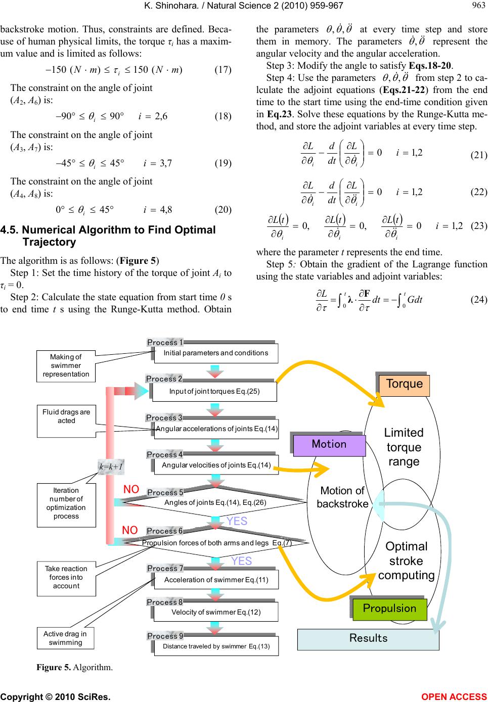

K. Shinohara. / Natural Science 2 (2010) 959-967

963

backstroke motion. Thus, constraints are defined. Beca-

use of human physical limits, the torque τi has a maxim-

um value and is limited as follows:

)(150)(150 mNmN i







(17)

The constraint on the angle of joint

(A2, A6) is:

6,29090  i



(18)

The constraint on the angle of joint

(A3, A7) is:

7,3 4545 i



(19)

The constraint on the angle of joint

(A4, A8) is:

8,4450  i



(20)

4.5. Numerical Algorithm to Find Optimal

Trajectory

The algorithm is as follows: (Figure 5)

Step 1: Set the time history of the torque of joint Ai to

τi = 0.

Step 2: Calculate the state equation from start time 0 s

to end time t s using the Runge-Kutta method. Obtain

the parameters



,, at every time step and store

them in memory. The parameters



, represent the

angular velocity and the angular acceleration.

Step 3: Modify the angle to satisfy Eqs.18-20.

Step 4: Use the parameters



,, from step 2 to ca-

lculate the adjoint equations (Eqs.21-22) from the end

time to the start time using the end-time condition given

in Eq.23. Solve these equations by the Runge-Kutta me-

thod, and store the adjoint variables at every time step.

2,10 



















i



 (21)

2,10 



















i



 (22)









2,10,0,0 











tLtLtL

iii



 (23)

where the parameter t represents the end time.

Step 5: Obtain the gradient of the Lagrange function

using the state variables and adjoint variables:

Ldt Gdt





 





λ (24)

Initial parameters and conditions

Angular accelerations of joints Eq.(14)

Angles of joints Eq.(14), Eq.(26)

Propulsion forces of both arms and legs Eq.(7)

Acceleration of swimmer Eq.(11)

Distance traveled by swimmer Eq.(13)

Motion of

backstroke

Limited

torque

range

Optimal

stroke

computing

Motion

To rq ue

Propulsion

Active drag in

swimming

Fluid drags are

acted

Making of

swimmer

representation

YES

Take reaction

forces into

account

Velocity of swimmer Eq.(12)

Angular velocities of joints Eq.(14)

Resul ts

Process 1

Process 3

Process 4

Process 5

Process 6

Process 7

Process 8

Process 9

Input of joint torques Eq.(25)

Process 2

k=k+1

Iteration

number of

optimization

process

Figure 5. Algorithm.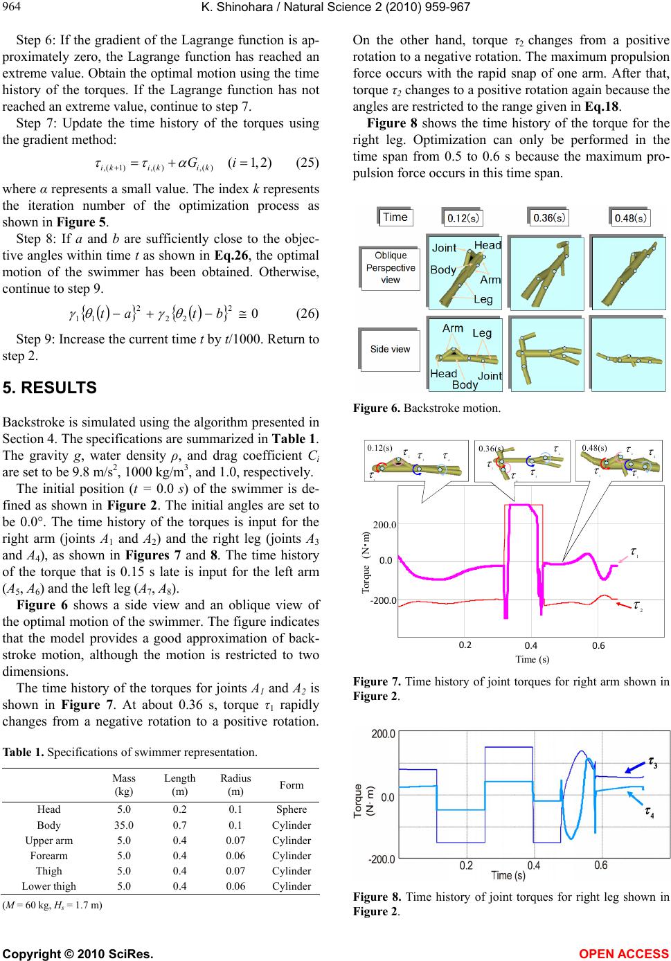

K. Shinohara / Natural Science 2 (2010) 959-967

964

Step 6: If the gradient of the Lagrange function is ap-

proximately zero, the Lagrange function has reached an

extreme value. Obtain the optimal motion using the time

history of the torques. If the Lagrange function has not

reached an extreme value, continue to step 7.

Step 7: Update the time history of the torques using

the gradient method:

,(1),( ),( )(1,2)

ik ikik







(25)

where α represents a small value. The index k represents

the iteration number of the optimization process as

shown in Figure 5.

Step 8: If a and b are sufficiently close to the objec-

tive angles within time t as shown in Eq.26, the optimal

motion of the swimmer has been obtained. Otherwise,

continue to step 9.







11 btat



(26)

Step 9: Increase the current time t by t/1000. Return to

step 2.

5. RESULTS

Backstroke is simulated using the algorithm presented in

Section 4. The specifications are summarized in Table 1.

The gravity g, water density ρ, and drag coefficient Ci

are set to be 9.8 m/s2, 1000 kg/m3, and 1.0, respectively.

The initial position (t = 0.0 s) of the swimmer is de-

fined as shown in Figure 2. The initial angles are set to

be 0.0°. The time history of the torques is input for the

right arm (joints A1 and A2) and the right leg (joints A3

and A4), as shown in Figures 7 and 8. The time history

of the torque that is 0.15 s late is input for the left arm

(A5, A6) and the left leg (A7, A8).

Figure 6 shows a side view and an oblique view of

the optimal motion of the swimmer. The figure indicates

that the model provides a good approximation of back-

stroke motion, although the motion is restricted to two

dimensions.

The time history of the torques for joints A1 and A2 is

shown in Figure 7. At about 0.36 s, torque τ1 rapidly

changes from a negative rotation to a positive rotation.

Table 1. Specifications of swimmer representation.

Mass

(kg)

Length

(m)

Radius

(m) Form

Head 5.0 0.2 0.1 Sphere

Body 35.0 0.7 0.1 Cylinder

Upper arm 5.0 0.4 0.07 Cylinder

Forearm 5.0 0.4 0.06 Cylinder

Thigh 5.0 0.4 0.07 Cylinder

Lower thigh 5.0 0.4 0.06 Cylinder

(M = 60 kg, Hs = 1.7 m)

On the other hand, torque τ2 changes from a positive

rotation to a negative rotation. The maximum propulsion

force occurs with the rapid snap of one arm. After that,

torque τ2 changes to a positive rotation again because the

angles are restricted to the range given in Eq.18.

Figure 8 shows the time history of the torque for the

right leg. Optimization can only be performed in the

time span from 0.5 to 0.6 s because the maximum pro-

pulsion force occurs in this time span.

Figure 6. Backstroke motion.

0.2

‐200.0

200.0

0.0

Torque (N・m)

0.12(s)

0.4 0.6

Time (s)



0.48(s)

0.36(s)

Figure 7. Time history of joint torques for right arm shown in

Figure 2.

Figure 8. Time history of joint torques for right leg shown in

Figure 2.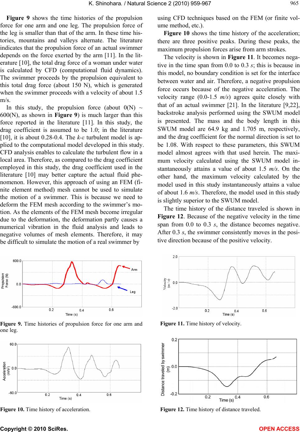

K. Shinohara. / Natural Science 2 (2010) 959-967

965

Figure 9 shows the time histories of the propulsion

force for one arm and one leg. The propulsion force of

the leg is smaller than that of the arm. In these time his-

tories, mountains and valleys alternate. The literature

indicates that the propulsion force of an actual swimmer

depends on the force exerted by the arm [11]. In the lit-

erature [10], the total drag force of a woman under water

is calculated by CFD (computational fluid dynamics).

The swimmer proceeds by the propulsion equivalent to

this total drag force (about 150 N), which is generated

when the swimmer proceeds with a velocity of about 1.5

m/s.

In this study, the propulsion force (about 0(N) ~

600(N), as shown in Figure 9) is much larger than this

force reported in the literature [11]. In this study, the

drag coefficient is assumed to be 1.0; in the literature

[10], it is about 0.28-0.4. The k-ε turbulent model is ap-

plied to the computational model developed in this study.

CFD analysis enables to calculate the turbulent flow in a

local area. Therefore, as compared to the drag coefficient

employed in this study, the drag coefficient used in the

literature [10] may better capture the actual fluid phe-

nomenon. However, this approach of using an FEM (fi-

nite element method) mesh cannot be used to simulate

the motion of a swimmer. This is because we need to

deform the FEM mesh according to the swimmer’s mo-

tion. As the elements of the FEM mesh become irregular

due to the deformation, the deformation partly causes a

numerical vibration in the fluid analysis and leads to

negative volumes of mesh elements. Therefore, it may

be difficult to simulate the motion of a real swimmer by

Figure 9. Time histories of propulsion force for one arm and

one leg.

Figure 10. Time history of acceleration.

using CFD techniques based on the FEM (or finite vol-

ume method, etc.).

Figure 10 shows the time history of the acceleration;

there are three positive peaks. During these peaks, the

maximum propulsion forces arise from arm strokes.

The velocity is shown in Figure 11. It becomes nega-

tive in the time span from 0.0 to 0.3 s; this is because in

this model, no boundary condition is set for the interface

between water and air. Therefore, a negative propulsion

force occurs because of the negative acceleration. The

velocity range (0.0-1.5 m/s) agrees quite closely with

that of an actual swimmer [21]. In the literature [9,22],

backstroke analysis performed using the SWUM model

is presented. The mass and the body length in this

SWUM model are 64.9 kg and 1.705 m, respectively,

and the drag coefficient for the normal direction is set to

be 1.08. With respect to these parameters, this SWUM

model almost agrees with that used herein. The maxi-

mum velocity calculated using the SWUM model in-

stantaneously attains a value of about 1.5 m/s. On the

other hand, the maximum velocity calculated by the

model used in this study instantaneously attains a value

of about 1.6 m/s. Therefore, the model used in this study

is slightly superior to the SWUM model.

The time history of the distance traveled is shown in

Figure 12. Because of the negative velocity in the time

span from 0.0 to 0.3 s, the distance becomes negative.

After 0.3 s, the swimmer consistently moves in the posi-

tive direction because of the positive velocity.

Figure 11. Time history of velocity.

Figure 12. Time history of distance traveled.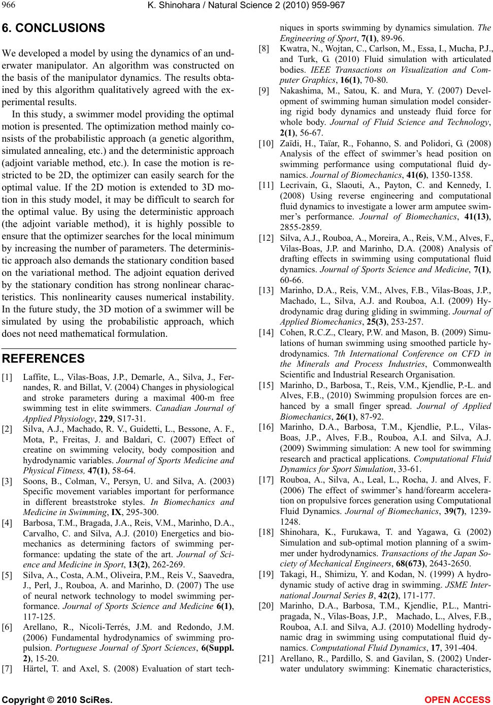

K. Shinohara / Natural Science 2 (2010) 959-967

966

6. CONCLUSIONS

We developed a model by using the dynamics of an und-

erwater manipulator. An algorithm was constructed on

the basis of the manipulator dynamics. The results obta-

ined by this algorithm qualitatively agreed with the ex-

perimental results.

In this study, a swimmer model providing the optimal

motion is presented. The optimization method mainly co-

nsists of the probabilistic approach (a genetic algorithm,

simulated annealing, etc.) and the deterministic approach

(adjoint variable method, etc.). In case the motion is re-

stricted to be 2D, the optimizer can easily search for the

optimal value. If the 2D motion is extended to 3D mo-

tion in this study model, it may be difficult to search for

the optimal value. By using the deterministic approach

(the adjoint variable method), it is highly possible to

ensure that the optimizer searches for the local minimum

by increasing the number of parameters. The determinis-

tic approach also demands the stationary condition based

on the variational method. The adjoint equation derived

by the stationary condition has strong nonlinear charac-

teristics. This nonlinearity causes numerical instability.

In the future study, the 3D motion of a swimmer will be

simulated by using the probabilistic approach, which

does not need mathematical formulation.

REFERENCES

[1] Laffite, L., Vilas-Boas, J.P., Demarle, A., Silva, J., Fer-

nandes, R. and Billat, V. (2004) Changes in physiological

and stroke parameters during a maximal 400-m free

swimming test in elite swimmers. Canadian Journal of

Applied Physiology, 229, S17-31.

[2] Silva, A.J., Machado, R. V., Guidetti, L., Bessone, A. F.,

Mota, P., Freitas, J. and Baldari, C. (2007) Effect of

creatine on swimming velocity, body composition and

hydrodynamic variables. Journal of Sports Medicine and

Physical Fitness, 47(1), 58-64.

[3] Soons, B., Colman, V., Persyn, U. and Silva, A. (2003)

Specific movement variables important for performance

in different breaststroke styles. In Biomechanics and

Medicine in Swimming, IX, 295-300.

[4] Barbosa, T.M., Bragada, J.A., Reis, V.M., Marinho, D.A.,

Carvalho, C. and Silva, A.J. (2010) Energetics and bio-

mechanics as determining factors of swimming per-

formance: updating the state of the art. Journal of Sci-

ence and Medicine in Sport, 13(2), 262-269.

[5] Silva, A., Costa, A.M., Oliveira, P.M., Reis V., Saavedra,

J., Perl, J., Rouboa, A. and Marinho, D. (2007) The use

of neural network technology to model swimming per-

formance. Journal of Sports Science and Medicine 6(1),

117-125.

[6] Arellano, R., Nicoli-Terrés, J.M. and Redondo, J.M.

(2006) Fundamental hydrodynamics of swimming pro-

pulsion. Portuguese Journal of Sport Sciences, 6(Suppl.

2), 15-20.

[7] Härtel, T. and Axel, S. (2008) Evaluation of start tech-

niques in sports swimming by dynamics simulation. The

Engineering of Sport, 7(1), 89-96.

[8] Kwatra, N., Wojtan, C., Carlson, M., Essa, I., Mucha, P.J.,

and Turk, G. (2010) Fluid simulation with articulated

bodies. IEEE Transactions on Visualization and Com-

puter Graphics, 16(1), 70-80.

[9] Nakashima, M., Satou, K. and Mura, Y. (2007) Devel-

opment of swimming human simulation model consider-

ing rigid body dynamics and unsteady fluid force for

whole body. Journal of Fluid Science and Technology,

2(1), 56-67.

[10] Zaïdi, H., Taïar, R., Fohanno, S. and Polidori, G. (2008)

Analysis of the effect of swimmer’s head position on

swimming performance using computational fluid dy-

namics. Journal of Biomechanics, 41(6), 1350-1358.

[11] Lecrivain, G., Slaouti, A., Payton, C. and Kennedy, I.

(2008) Using reverse engineering and computational

fluid dynamics to investigate a lower arm amputee swim-

mer’s performance. Journal of Biomechanics, 41(13),

2855-2859.

[12] Silva, A.J., Rouboa, A., Moreira, A., Reis, V.M., Alves, F.,

Vilas-Boas, J.P. and Marinho, D.A. (2008) Analysis of

drafting effects in swimming using computational fluid

dynamics. Journal of Sports Science and Medicine, 7(1),

60-66.

[13] Marinho, D.A., Reis, V.M., Alves, F.B., Vilas-Boas, J.P.,

Machado, L., Silva, A.J. and Rouboa, A.I. (2009) Hy-

drodynamic drag during gliding in swimming. Journal of

Applied Biomechanics, 25(3), 253-257.

[14] Cohen, R.C.Z., Cleary, P.W. and Mason, B. (2009) Simu-

lations of human swimming using smoothed particle hy-

drodynamics. 7th International Conference on CFD in

the Minerals and Process Industries, Commonwealth

Scientific and Industrial Research Organisation.

[15] Marinho, D., Barbosa, T., Reis, V.M., Kjendlie, P.-L. and

Alves, F.B., (2010) Swimming propulsion forces are en-

hanced by a small finger spread. Journal of Applied

Biomechanics, 26(1), 87-92.

[16] Marinho, D.A., Barbosa, T.M., Kjendlie, P.L., Vilas-

Boas, J.P., Alves, F.B., Rouboa, A.I. and Silva, A.J.

(2009) Swimming simulation: A new tool for swimming

research and practical applications. Computational Fluid

Dynamics for Sport Simulation, 33-61.

[17] Rouboa, A., Silva, A., Leal, L., Rocha, J. and Alves, F.

(2006) The effect of swimmer’s hand/forearm accelera-

tion on propulsive forces generation using Computational

Fluid Dynamics. Journal of Biomechanics, 39(7), 1239-

1248.

[18] Shinohara, K., Furukawa, T. and Yagawa, G. (2002)

Simulation and sub-optimal motion planning of a swim-

mer under hydrodynamics. Transactions of the Japan So-

ciety of Mechanical Engineers, 68(673), 2643-2650.

[19] Takagi, H., Shimizu, Y. and Kodan, N. (1999) A hydro-

dynamic study of active drag in swimming. JSME Inter-

national Journal Series B, 42(2), 171-177.

[20] Marinho, D.A., Barbosa, T.M., Kjendlie, P.L., Mantri-

pragada, N., Vilas-Boas, J.P., Machado, L., Alves, F.B.,

Rouboa, A.I. and Silva, A.J. (2010) Modelling hydrody-

namic drag in swimming using computational fluid dy-

namics. Computational Fluid Dynamics, 17, 391-404.

[21] Arellano, R., Pardillo, S. and Gavilan, S. (2002) Under-

water undulatory swimming: Kinematic characteristics,

K. Shinohara. / Natural Science 2 (2010) 959-967

967

vortex generation and application during the start, turn

and swimming strokes. Proceedings of the 20th Interna-

tional Symposium on Biomechanics in Sports, Universi-

dad de Granada.

[22] Nakashima, M. (2007) Analysis of breast, back and but-

terfly strokes by the swimming human simulation model

swum. In: Kato, N. and Kamimura, S., Eds., Biomecha-

nisms of Animals in Swimming and Flying-Fluid Dynam-

ics, Biomimetic Robots, and Sports Science, Springer-

Verlag, 361-367.