General Scattering Mechanism and Transport in Graphene

doi:10.4236/graphene.2013.21007

Paper Menu >>

Journal Menu >>

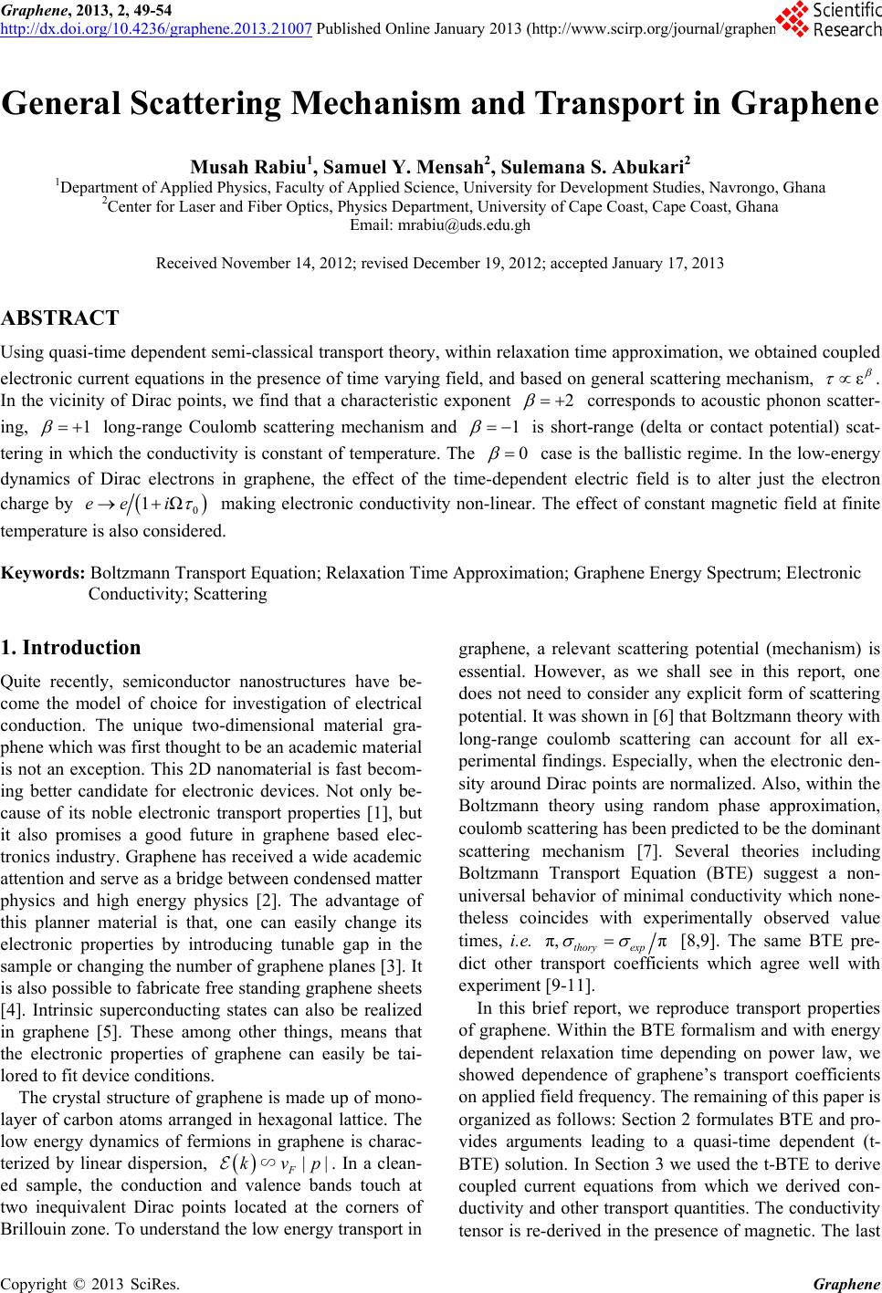Graphene, 2013, 2, 49-54

http://dx.doi.org/10.4236/graphene.2013.21007 Published Online January 2013 (http://www.scirp.org/journal/graphene)

General Scattering Mechanism and Transport in Graphene

Musah Rabiu1, Samuel Y. Mensah2, Sulemana S. Abukari2

1Department of Applied Physics, Faculty of Applied Science, University for Development Studies, Navrongo, Ghana

2Center for Laser and Fiber Optics, Physics Department, University of Cape Coast, Cape Coast, Ghana

Email: [email protected]

Received November 14, 2012; revised December 19, 2012; accepted January 17, 2013

ABSTRACT

Using quasi-time dependent semi-classical transport theory, within relaxation time approximation, we obtained coupled

electronic current equations in the presence of time varying field, and based on general scattering mechanism, ε





.

In the vicinity of Dirac points, we find that a characteristic exponent 2





 corresponds to acoustic phonon scatter-

ing, 1



 long-range Coulomb scattering mechanism and 1





 is short-range (delta or contact potential) scat-

tering in which the conductivity is constant of temperature. The 0





case is the ballistic regime. In the low-energy

dynamics of Dirac electrons in graphene, the effect of the time-dependent electric field is to alter just the electron

charge by



1Ωee i



 making electronic conductivity non-linear. The effect of constant magnetic field at finite

temperature is also considered.

Keywords: Boltzmann Transport Equation; Relaxation Time Approximation; Graphene Energy Spectrum; Electronic

Conductivity; Scattering

1. Introduction

Quite recently, semiconductor nanostructures have be-

come the model of choice for investigation of electrical

conduction. The unique two-dimensional material gra-

phene which was first thought to be an academic material

is not an exception. This 2D nanomaterial is fast becom-

ing better candidate for electronic devices. Not only be-

cause of its noble electronic transport properties [1], but

it also promises a good future in graphene based elec-

tronics industry. Graphene has received a wide academic

attention and serve as a bridge between condensed matter

physics and high energy physics [2]. The advantage of

this planner material is that, one can easily change its

electronic properties by introducing tunable gap in the

sample or changing the number of graphene planes [3]. It

is also possible to fabricate free standing graphene sheets

[4]. Intrinsic superconducting states can also be realized

in graphene [5]. These among other things, means that

the electronic properties of graphene can easily be tai-

lored to fit device conditions.

The crystal structure of graphene is made up of mono-

layer of carbon atoms arranged in hexagonal lattice. The

low energy dynamics of fermions in graphene is charac-

terized by linear dispersion,





kv|p∽

graphene, a relevant scattering potential (mechanism) is

essential. However, as we shall see in this report, one

does not need to consider any explicit form of scattering

potential. It was shown in [6] that Boltzmann theory with

long-range coulomb scattering can account for all ex-

perimental findings. Especially, when the electronic den-

sity around Dirac points are normalized. Also, within the

Boltzmann theory using random phase approximation,

coulomb scattering has been predicted to be the dominant

scattering mechanism [7]. Several theories including

Boltzmann Transport Equation (BTE) suggest a non-

universal behavior of minimal conductivity which none-

theless coincides with experimentally observed value

times, i.e. π,π

thory exp





 [8,9]. The same BTE pre-

dict other transport coefficients which agree well with

experiment [9-11].

In this brief report, we reproduce transport properties

of graphene. Within the BTE formalism and with energy

dependent relaxation time depending on power law, we

showed dependence of graphene’s transport coefficients

on applied field frequency. The remaining of this paper is

organized as follows: Section 2 formulates BTE and pro-

vides arguments leading to a quasi-time dependent (t-

BTE) solution. In Section 3 we used the t-BTE to derive

coupled current equations from which we derived con-

ductivity and other transport quantities. The conductivity

tensor is re-derived in the presence of magnetic. The last

|. In a clean-

ed sample, the conduction and valence bands touch at

two inequivalent Dirac points located at the corners of

Brillouin zone. To understand the low energy transport in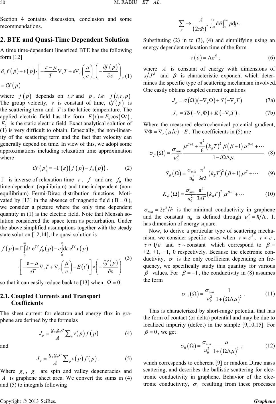

M. RABIU ET AL.

Section 4 contains discussion, conclusion and some

recommendations.

2. BTE and Quasi-Time Dependent Solution

A time time-dependent linearized BTE has the following

form [12]

 







trr

fp vpTe

 





 



 















, (1)

where



p depends on and , i.e. t,r p





t,r,p

The group velocity, is constant of time, v





p is

the scattering term and is the lattice temperature. The

applied electric field has the form







0cos ΩE tEt,

0 is the static electric field. Exact analytical solution of

(1) is very difficult to obtain. Especially, the non-linear-

ity of the scattering term and the fact that velocity can

generally depend on time. In view of this, we adopt some

approximations including relaxation time approximation

where

 





pfpf



 p. (2)

Γ is inverse of relaxation time



and are 0

the

time-dependent (equilibrium) and time-independent (non-

equilibrium) Fermi-Dirac distribution functions. Moti-

vated by [13] in the absence of magnetic field (B0



we consider a picture where the only time dependent

quantity in (1) is the electric field. Note that Mensah so-

lution considered the space term as perturbation. Under

the above simplified assumptions together with the steady

state solution [12,14], the quasi solution is

 

 

ΓΓ

Γd ed e

fptf petvp

TEt

eT e













 

 

 















(3)

so that it can easily reduce back to [13] when Ω0



2.1. Coupled Currents and Transport

Coefficients

The sheet current for electron and energy flux in gra-

phene are defined by the formulas



gge

vpfp

 (4)

and



sv p

gge

pfp



. (5)

Where

, v

are spin and valley degeneracies and

is graphene sheet area. We convert the sums in (4)

and (5) to integrals following



2π0

2π-

App











Substituting (2) in to (3), (4) and simplifying using an

energy dependent relaxation time of the form





Λε





, (6)

where

is constant of energy with dimensions of



and



is characteristic exponent which deter-

mines the specific type of scattering mechanism involved.

One easily obtains coupled current equations













ΩΦ

err





(7a)







TSK T



. (7b)

Where the measured electrochemical potential gradient,





ΦreE





 . The coefficients in (5) are

  

π1

Ω

1ΩΛ

min kT





















(8)

  

Ω1

min B

SkT







 (9)

 

221

Ω

min B

KkT









 (10)

min eh



 is the minimal conductivity in graphene

and the constant 0 is defined through u2

0Λu. It

has dimension of energy square.

Now, to derive a particular type of scattering mecha-

nism, we consider specific cases when 2





,













and constant





which correspond to



+2, +1, −1, 0 respectively. Because the electronic con-

ductivity,



is the only coefficient depending on fre-

quency, we specifically study this quantity for various



values. For 1





, the conductivity in (8) assumes

the form

 

Ω

1ΩΛ

min





. (11)

This is characterized by short-range potential that has

the form of contact (or delta) potential and may be due to

localized impurity (defect) in the sample [9,10,15]. For





, we get

 

Ω

1ΩΛ

min







, (12)

which corresponds to coherent [9] or random Dirac mass

scattering, and describes the ballistic scattering for elec-

tronic conductivity in graphene. Behavior of the elec-

tronic conductivity, 0



resulting from these processes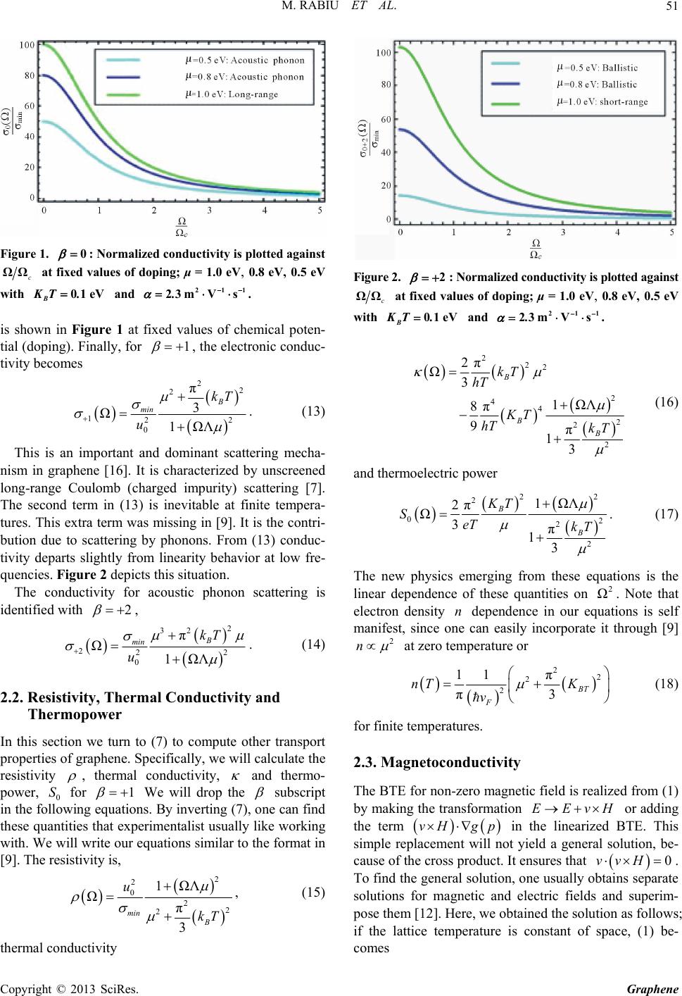

M. RABIU ET AL. 51

Figure 1. 0



: Normalized conductivity is plotted against

ΩΩ at fixed values of doping; μ = 1.0 eV, 0.8 eV, 0.5 eV

with and . .0 1 e

KT V21

23m Vs.





1

is shown in Figure 1 at fixed values of chemical poten-

tial (doping). Finally, for 1



 , the electronic conduc-

tivity becomes

 



Ω

1ΩΛ

min kT









2

. (13)

This is an important and dominant scattering mecha-

nism in graphene [16]. It is characterized by unscreened

long-range Coulomb (charged impurity) scattering [7].

The second term in (13) is inevitable at finite tempera-

tures. This extra term was missing in [9]. It is the contri-

bution due to scattering by phonons. From (13) conduc-

tivity departs slightly from linearity behavior at low fre-

quencies. Figure 2 depicts this situation.

The conductivity for acoustic phonon scattering is

identified with 2



 ,

 



Ω

1ΩΛ

min kT









. (14)

2.2. Resistivity, Thermal Conductivity and

Thermopower

In this section we turn to (7) to compute other transport

properties of graphene. Specifically, we will calculate the

resistivity



, thermal conductivity, and thermo-

power, 0 for





 We will drop the



subscript

in the following equations. By inverting (7), one can find

these quantities that experimentalist usually like working

with. We will write our equations similar to the format in

[9]. The resistivity is,









1ΩΛ

Ω

min B











, (15)

thermal conductivity

Figure 2. 2





: Normalized conductivity is plotted against

ΩΩ at fixed values of doping; μ = 1.0 eV, 0.8 eV, 0.5 eV

with and .

KT V.01e

23mVs.





1

 



222

2π

Ω

1ΩΛ

8π

9π

hT kT













(16)

and thermoelectric power

  



1ΩΛ

2π

Ω

3π

SeT kT









. (17)

The new physics emerging from these equations is the

linear dependence of these quantities on . Note that

electron density dependence in our equations is self

manifest, since one can easily incorporate it through [9]

Ω



 at zero temperature or

  

11 π

π3BT

nT K













(18)

for finite temperatures.

2.3. Magnetoconductivity

The BTE for non-zero magnetic field is realized from (1)

by making the transformation or adding

the term

EEvH









vH gp in the linearized BTE. This

simple replacement will not yield a general solution, be-

cause of the cross product. It ensures that .

To find the general solution, one usually obtains separate

solutions for magnetic and electric fields and superim-

pose them [12]. Here, we obtained the solution as follows;

if the lattice temperature is constant of space, (1) be-

comes



0H vv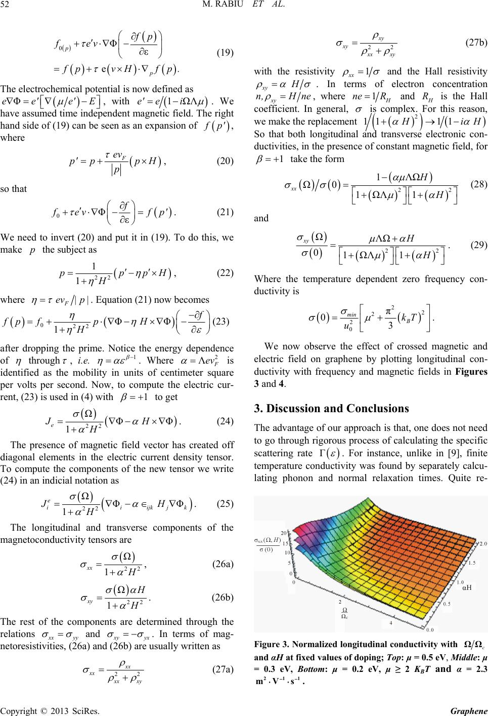

M. RABIU ET AL.



 

0Φ

fev

pvHf















p.

(19)

The electrochemical potential is now defined as



Φee' e'E



 





, with



1ΩΛe' ei



 . We

have assumed time independent magnetic field. The right

hand side of (19) can be seen as an expansion of





p' ,

where



p'pp H



 



(20)

so that



0Φ

evf p'















 . (21)

We need to invert (20) and put it in (19). To do this, we

make the subject as



ppp













, (22)

where F

ev| p|





. Equation (21) now becomes

 

022 Φ Φ

fp fpH











 







(23)

after dropping the prime. Notice the energy dependence



through



, i.e. 1









. Where 2



 is

identified as the mobility in units of centimeter square

per volts per second. Now, to compute the electric cur-

rent, (23) is used in (4) with 1



 to get



Ω

Φ Φ







H. (24)

The presence of magnetic field vector has created off

diagonal elements in the electric current density tensor.

To compute the components of the new tensor we write

(24) in an indicial notation as



Ω

iiijk







Φ

. (25)

The longitudinal and transverse components of the

magnetoconductivity tensors are





Ω





, (26a)



Ω







. (26b)

The rest of the components are determined through the

relations

xyy



 and

yyx





. In terms of mag-

netoresistivities, (26a) and (26b) are usually written as

xxy







 (27a)

xxy







 (27b)

with the resistivity 1







and the Hall resistivity

xy H







. In terms of electron concentration

n,H ne





, where 1

ne R



and

R is the Hall

coefficient. In general,



is complex. For this reason,

we make the replacement



11 1

1 iH





So that both longitudinal and transverse electronic con-

ductivities, in the presence of constant magnetic field, for





 take the form

 

 

1ΛΩ

Ω0

1ΩΛ 1



 







 





 

(28)

and





  

ΩΛΩ

01ΩΛ1

xy H





2



 





 

. (29)

Where the temperature dependent zero frequency con-

ductivity is

 

min B

















.

We now observe the effect of crossed magnetic and

electric field on graphene by plotting longitudinal con-

ductivity with frequency and magnetic fields in Figures

3 and 4.

3. Discussion and Conclusions

The advantage of our approach is that, one does not need

to go through rigorous process of calculating the specific

scattering rate







. For instance, unlike in [9], finite

temperature conductivity was found by separately calcu-

lating phonon and normal relaxation times. Quite re-

Figure 3. Normalized longitudinal conductivity with c

ΩΩ

and αH at fixed values of doping; Top: μ = 0.5 eV, Middle: μ

= 0.3 eV, Bottom: μ = 0.2 eV, μ ≥ 2 KBT and α = 2.3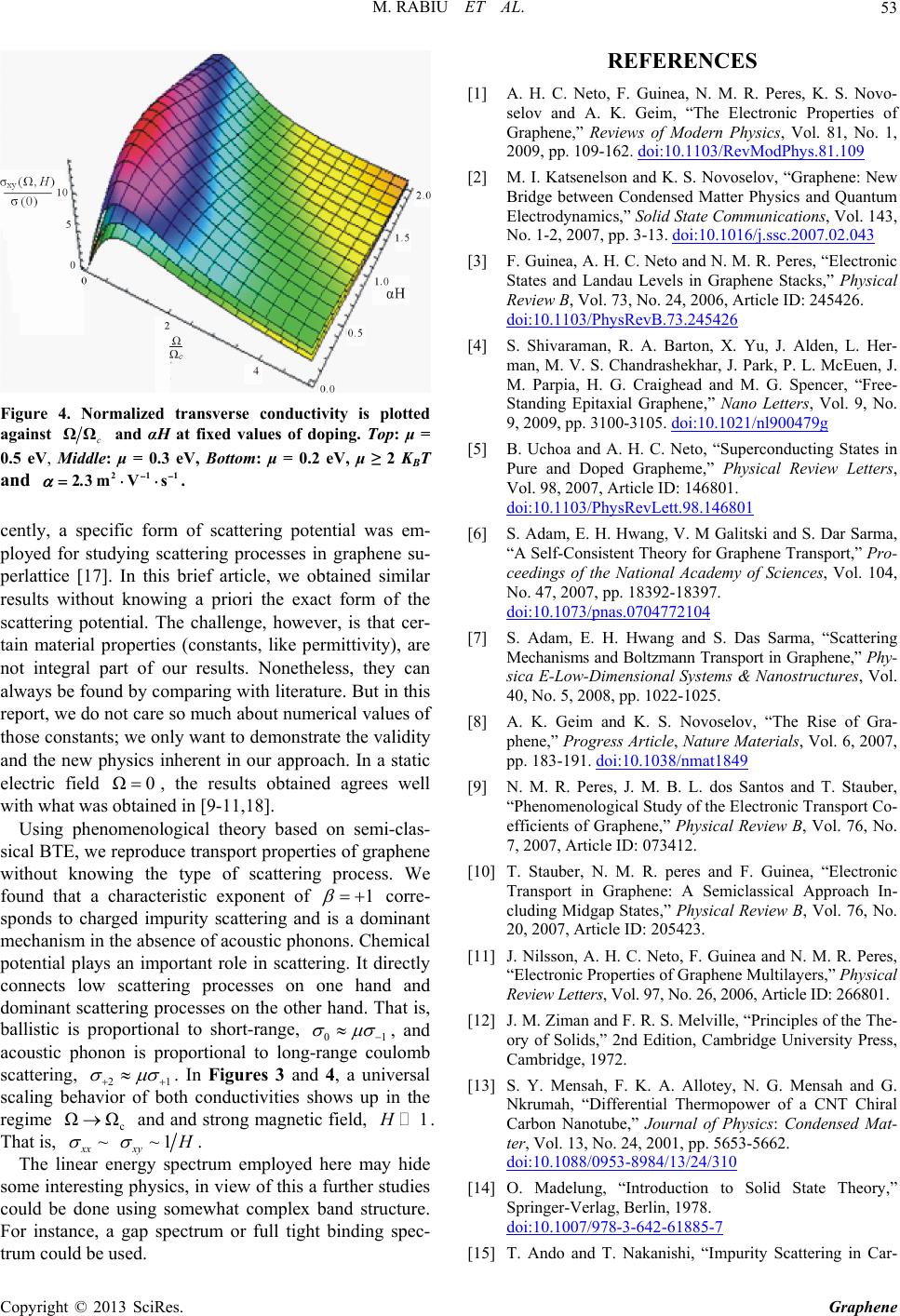

mVs





.

M. RABIU ET AL. 53

Figure 4. Normalized transverse conductivity is plotted

against c

ΩΩ and αH at fixed values of doping. Top: μ =

0.5 eV, Middle: μ = 0.3 eV, Bottom: μ = 0.2 eV, μ ≥ 2 KBT

and 211

23mVs.





.

cently, a specific form of scattering potential was em

ain

ased on semi-clas-

ployed for studying scattering processes in graphene su-

perlattice [17]. In this brief article, we obtained similar

results without knowing a priori the exact form of the

scattering potential. The challenge, however, is that cer-

tain material properties (constants, like permittivity), are

not integral part of our results. Nonetheless, they can

always be found by comparing with literature. But in this

report, we do not care so much about numerical values of

those constants; we only want to demonstrate the validity

and the new physics inherent in our approach. In a static

electric field Ω0, the results obtained agrees well

with what was obted in [9-11,18].

Using phenomenological theory b

cal BTE, we reproduce transport properties of graphene

without knowing the type of scattering process. We

found that a characteristic exponent of 1



 corre-

sponds to charged impurity scattering and minant

mechanism in the absence of acoustic phonons. Chemical

potential plays an important role in scattering. It directly

connects low scattering processes on one hand and

dominant scattering processes on the other hand. That is,

ballistic is proportional to short-range, 01

is a do







, and

acoustic phonon is proportional to long-lomb

scattering, 21

range cou







. In Figures 3 and 4, a universal

scaling behth conductivities shows up in the

regime c

ΩΩ and and strong magnetic field, 1

avior of bo



That is, 1

xy ~H

xx ~



near ene

The litrurgy specm employ

trum could be used.

. Guinea, N. M. R. Peres, K. S. Novo-

selov and A. K. Geim, “The Electronic Properties of

Graphene,” Re, Vol. 81, No. 1,

2009, pp. 109-dPhys.81.109

ed yhere ma hide

me interesting physics, in view of this a further studies

could be done using somewhat complex band structure.

For instance, a gap spectrum or full tight binding spec-

REFERENCES

[1] A. H. C. Neto, F

views of Modern Physics

162. doi:10.1103/RevMo

[2] M. I. Katsenelson and K. S. Novoselov, “Graphene: New

Bridge between Condensed Matter Physics and Quantum

Electrodynamics,” Solid State Communications, Vol. 143,

No. 1-2, 2007, pp. 3-13. doi:10.1016/j.ssc.2007.02.043

[3] F. Guinea, A. H. C. Neto and N. M. R. Peres, “Electronic

States and Landau Levels in Graphene Stacks,” Physical

Review B, Vol. 73, No. 24, 2006, Article ID: 245426.

doi:10.1103/PhysRevB.73.245426

[4] S. Shivaraman, R. A. Barton, X. Yu, J. Alden, L. Her-

man, M. V. S. Chandrashekhar, J. Park, P. L. McEuen, J.

M. Parpia, H. G. Craighead and M. G. Spencer, “F

Standing Epitaxial Graphene,” Nan ree-

o Letters, Vol. 9, No.

9, 2009, pp. 3100-3105. doi:10.1021/nl900479g

[5] B. Uchoa and A. H. C. Neto, “Superconducting States in

Pure and Doped Grapheme,” Physical Review Letters,

Vol. 98, 2007, Article ID: 146801.

doi:10.1103/PhysRevLett.98.146801

[6] S. Adam, E. H. Hwang, V. M Galitski and S. Dar Sarma,

“A Self-Consistent Theory for Graphene Transport,” Pro-

ceedings of the National Academy of

No. 47, 2007, pp. 18392-18397.

Sciences, Vol. 104,

doi:10.1073/pnas.0704772104

[7] S. Adam, E. H. Hwang and S. Das Sarma, “Scattering

Mechanisms and Boltzmann Transport in Graphene,” Phy-

sica E-Low-Dimensional Systems

40, No. 5, 2008, pp. 1022-1025.

& Nanostructures, Vol.

[8] A. K. Geim and K. S. Novoselov, “The Rise of Gra-

phene,” Progress Article, Nature Materials, Vol. 6, 2007,

pp. 183-191. doi:10.1038/nmat1849

[9] N. M. R. Peres, J. M. B. L. dos Santos and T. Stauber,

“Phenomenological Study of the Electronic Transport Co-

efficients of Graphene,” Physical Review B, Vol. 76, No.

7, 2007, Article ID: 073412.

[10] T. Stauber, N. M. R. peres and F. Guinea, “Electronic

Transport in Graphene: A Semiclassical Approach In-

cluding Midgap States,” Physical Review B, Vol. 76, No.

20, 2007, Article ID: 205423.

[11] J. Nilsson, A. H. C. Neto, F. Guinea and N. M. R. Peres,

“Electronic Properties of Graphene Multilayers,” Physical

Review Letters, Vol. 97, No. 26, 2006, Article ID: 266801.

[12] J. M. Ziman and F. R. S. Melville, “Principles of the The-

ory of Solids,” 2nd Edition, Cambridge University Press,

Cambridge, 1972.

S. Y. Mensah, F. K. A. Allotey, N. G. Mensah and G.[13]

Nkrumah, “Differential Thermopower of a CNT Chiral

Carbon Nanotube,” Journal of Physics: Condensed Mat-

ter, Vol. 13, No. 24, 2001, pp. 5653-5662.

doi:10.1088/0953-8984/13/24/310

[14] O. Madelung, “Introduction to Solid State Theory,”

Springer-Verlag, Berlin, 1978.

doi:10.1007/978-3-642-61885-7

[15] T. Ando and T. Nakanishi, “Impurity Scattering in Car-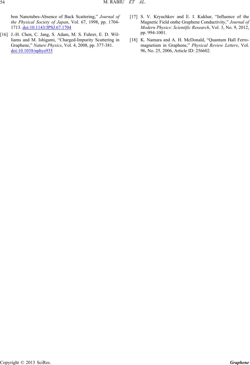

M. RABIU ET AL.

, pp. 1704-

bon Nanotubes-Absence of Back Scattering,” Journal of

the Physical Society of Japan, Vol. 67, 1998

1713. doi:10.1143/JPSJ.67.1704

[16] J.-H. Chen, C. Jang, S. Adam, M. S. Fuhrer, E. D. Wil-

liams and M. Ishigami, “Charged-Impurity Scattering in

Graphene,” Nature Physics, Vol. 4, 2008, pp. 377-381.

doi:10.1038/nphys935

[17] S. V. Kryuchkov and E. I. Kukhar, “Influence of the

Magnetic Field onthe G

raphene Conductivity,” Journal of

raphene,” Physical Review Letters, Vol.

Modern Physics: Scientific Research, Vol. 3, No. 9, 2012,

pp. 994-1001.

[18] K. Namura and A. H. McDonald, “Quantum Hall Ferro-

magnetism in G

96, No. 25, 2006, Article ID: 256602.