Portfolio Selection by Maximizing Omega Function using Differential Evolution

doi:10.4236/ti.2013.41B012

Paper Menu >>

Journal Menu >>

Technology and Investment, 2013, 4, 73-77

Published Online Febr uary 20 http://www.SciRP.org/journal/ti)

Portfolio Selection by Maximizing Omega Function using

Differential Evolution

PEKÁR Juraj, BREZINA Ivan, ČIČKOVÁ Zuzana, REIFF Marian

Department of Operations Research and Econometrics, University of Economics, Bratislava, Slovakia

Email: [email protected]

Received 2012

ABSTRACT

Paper presents alternative solution seeking approach for portfolio selection problem with Omega function performance

measure which allows determining capital allocation over the number of assets. Omega function computability is diffi-

cult due to substandard structures and therefore the use of standard techniques seems to be relatively complicated. Dif-

ferential evolution from the group of evolutionary algorithms was selected as an alternative computing procedure. Al-

ternative approach is analyzed on the Down Jones Industrial Index data. Presented approach enables to determine good

real-time solution and the quality of results is comparable with results obtained by professional software.

Keywords: differential evolution, Omega function, problem of portfolio selection

1. Introduction

In general, portfolio theory deals with the selection of an

appropriate mix of assets in a portfolio in order to meet

predetermined properties. Various mathematical models,

which measure the portfolio performance measurement

can be used to support the decision making process of

selection of the portfolio assets. The aim is to determine

the allocation of the available resources in the selected

group of assets that results in maximization of portfolio

performance. Follow this idea, various measurements of

performance can be used. The performance measurement

techniques are e.g. Sharpe ratio, Treynor ratio, Jensen's

alpha, Information Ratio, Sortino ratio, Omega function

and the Sharpe Omega ratio ([1], [2], [3], [4], [5], [6], [7],

[8]). The paper deals wi th Omega function, which com-

putability is difficult due to substandard structures of

performance level and therefore the use of standard tech-

niques seems to be relatively complicated. The alterna-

tive computing procedures includes variety of different

approaches. Nowadays a lot of research attention is fo-

cused on evolutionary algorithms. The paper presents the

algorithm of differential evolution that is able to deal

with nonlinear objective function with success (e na b l es

quick a c hieve ment of suboptimal solutions) and thus

demonstrates suitability of evolutionary algorithms for

financial modeling. Above mentioned approach is ana-

lyzed on assets inc lude d in the Down Jones Industrial

Inde x and its historical data1

publ is hed from July 1st

2001 to April 1st 2012 on weekly basis were used.

http://finance. yahoo. co m/ (2012)

2. Portfolio selection models based on

Omega function

Omega function is measure which incorporates all the

distributional, characteristics of a return series. The

measure is a function of the returns leveled and requires

no parametric assumption on the distribution. Precisely,

it considers the returns below and above a specific loss

threshold and provides a ratio of total probability

weighted losses and gains that fully describes the risk

reward properties of the distribution [8]:

where:

MAR denotes the return level regarded as a loss threshold,

(a, b ) denotes yields range,

F(x) the cumulative distribution fu nction of asset returns.

In the next part we formulate the problem of portfolio

selection based on omega function performance measure.

As it is mentioned, the Omega function involves consid-

eration of all the information contained in the time series

of returns. The aim of portfolio selection problem is to

maximize the level of Omega performance measure,

where the variables w1, w2,…wd (where d represents the

number of assets) represent the weights of each asset in

the portfolio. Corresponding problem can be formulated

as follows [9]:

∫

∫−

=Ω MAR

MAR

dxxF

MAR

)(

))(1(

)(

13 (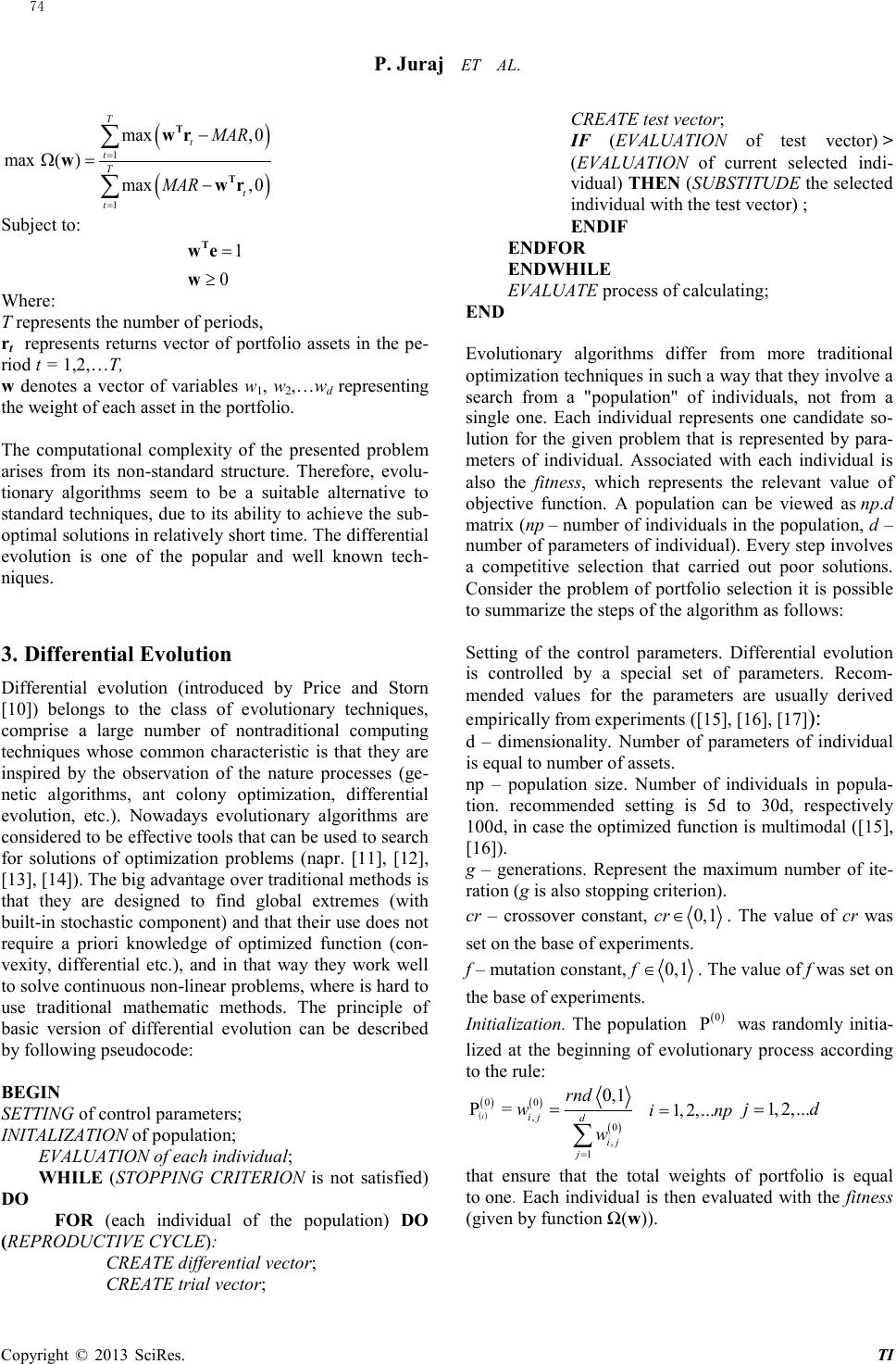

P. Juraj ET AL.

(

)

( )

max ,0

max( )

max ,0

MAR

−

Ω=

−

∑

Subject to:

≥

Wher e :

T represents the number of periods,

rt represents returns vector of portfolio assets in the pe-

riod t = 1,2,…T,

w denotes a vector of variables w1, w2,…wd representing

the weight of each asset in the portfolio.

The computationa l c omplexity of the presented problem

arises from its non-standard structure. Therefore, evolu-

tionary algorithms seem to be a suitable alternative to

standard techniques, due to its ability to achieve the sub-

optimal solutions in relatively short time. The d iffere ntial

evolution is one of the popular and well known tech-

niques.

3. Differential Evolution

Differential evolution (introduced by Price and Storn

[10]) belongs to the class of evolutionary techniques,

comprise a large number of nontraditional computing

techniques whose common characteristic is that they are

inspired by the observation of the nature processes (ge-

netic algorithms, ant colony optimization, differential

evolution, etc.). Nowadays evolutionary algorithms are

considered to be effective tools that can be used to search

for solutions of optimization problems (napr. [11], [12],

[13], [14]). The big advantage over traditional methods is

that they are designed to find global extremes (with

built-in stochastic component) and that their use does not

require a priori knowledge of optimized function (con-

vexity, differential etc.), and in that way they work well

to solve continuous non-linear problems, where is hard to

use traditional mathematic methods. The principle of

basic version of differential evolution can be described

by following pseudocode:

BEGIN

SETTING of control parameters;

INITALIZATION of population;

EVALUATION of each individual;

WHILE (STOPPING CRITERION is not satisfied)

FOR (each individual of the population) DO

(REPRODUCTIVE CYCLE):

CREATE differential vector;

CREATE trial vector;

CREATE test vector;

IF (EVALUATION of test vector) >

(EVALUATION of current selected indi-

vidual ) THEN (SUBSTITUD E the selected

individual with the test vector) ;

ENDIF

ENDFOR

ENDWHILE

EVALUATE process of calculating;

END

Evolutionary algorithms differ from more traditional

optimization techniques in such a way that they involve a

search from a "population" of individuals, not from a

single one. Each individual represents one candidate so-

lution for the given problem that is represented by para-

meters of individual. Associated with each individual is

also the fitness, which represents the relevant value of

objective function. A population can be viewed as np.d

matrix (np – number of individuals in the population, d –

number of parameters of individual). Every step involves

a competitive selection that carried out poor solutions.

Consider the problem of portfolio selection it is possible

to summarize the steps of the algorithm as follows:

Setting of the control parameters. Differential evolution

is controlled by a special set of parameters. Recom-

mended values for the parameters are usually derived

empirically from experiments ([15], [16], [17]):

d – dimensio na lity. Number of parameters of individual

is equal to number of asse ts.

np – population size. Number of individuals in popula-

tion. recommended setting is 5d to 30d, respectively

100d, in case the optimized function is multimodal ([15],

[16]).

g – generations. Represent the maximum number of ite-

ration (g is also stopping criterion).

cr – crossover constant, cr

0,1∈

. The value of cr was

set on the base of experiments.

f – mutation constant, f

0,1∈

. The value of f was set on

the base of experiments.

Initializatio n. The population

( )

was randomly initia-

lized at the beginning of evolutionary process according

to the rule:

( )

( )( )

( )

0,1

P =

ij d

rnd

=∑

1,2,...i np=

1,2, ...jd=

that ensure that the total weights of portfolio is equal

to one. Each individual is then evaluated with the fitne ss

(given by function Ω(w)).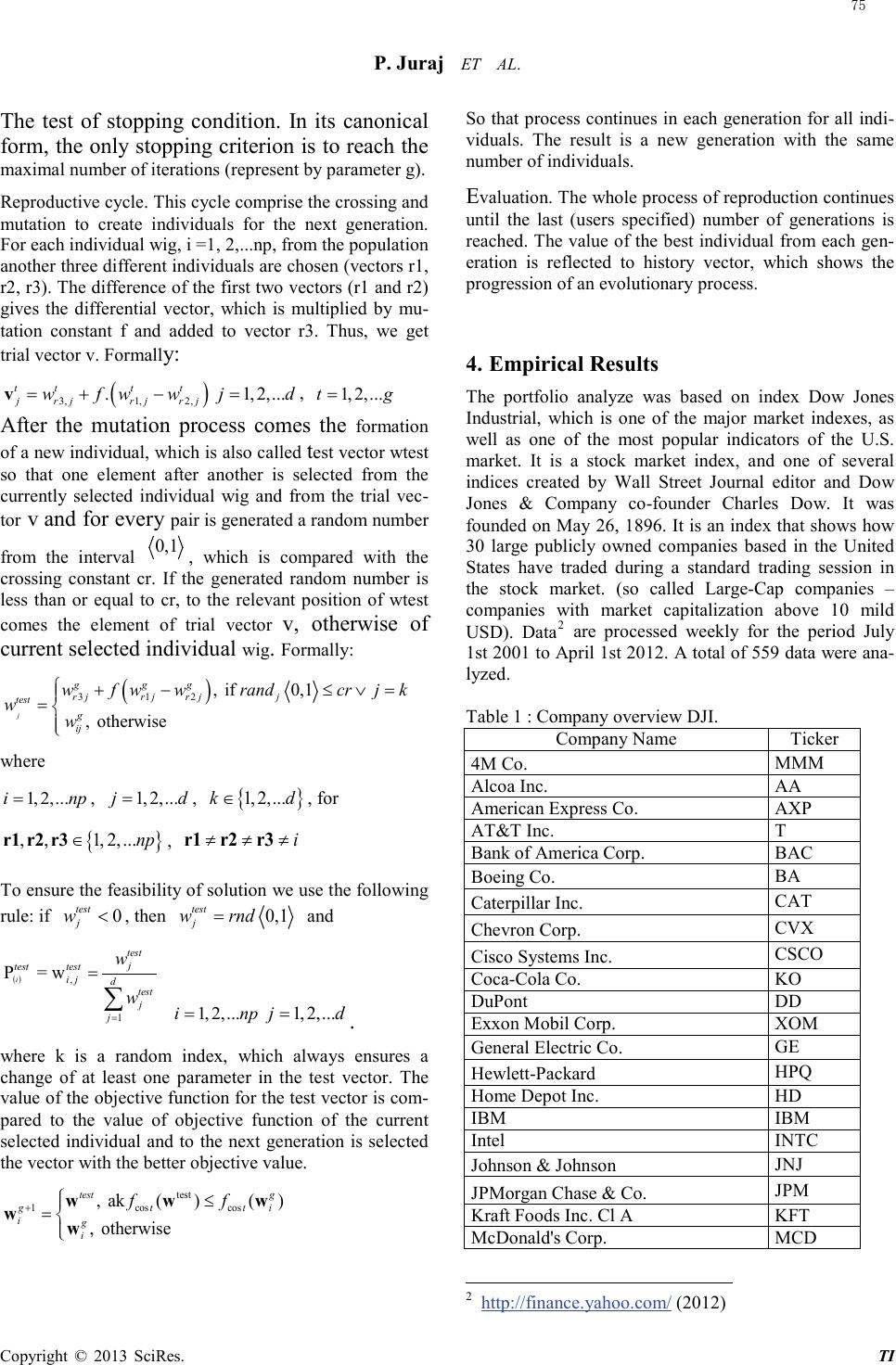

P. Juraj ET AL.

The test of stopping condition. In its canonical

form, the only stopping criterion is to reach the

maximal number of iterations (represent by parameter g).

Reproductive cycle. This cycle comprise the crossing and

mutation to create individuals for the next generation.

For each individual wig, i =1, 2,...np, from the population

another three different individuals are chosen (vectors r1,

r2, r3). The difference of the first two vectors (r1 and r2)

gives the differential vector, which is multiplied by mu-

tation constant f and added to vector r3. Thus, we get

trial vector v. Formally:

( )

3,1, 2,

ttt t

jr jrjrj

wfw w=+−v

1,2, ...jd=

1,2,...tg=

After the mutation process comes the formation

of a new individual, which is also called test vector wtest

so that one element after another is selected from the

currently selected individual wig and from the trial vec-

tor v and for every pair is generated a random number

from the interval

0,1

, which is compared with the

crossing constant cr. If the generated random number is

less than or equal to cr, to the relevant position of wtest

comes the element of trial vector v, otherwise of

current selected individual wig . Formal ly :

( )

3 12

, if 0,1

, otherwise

g gg

r jrjr jj

test

wf wwrandcrjk

+−≤ ∨=



=





where

1,2,...i np=

1,2, ...jd=

{ }

1,2, ...kd∈

, for

{ }

,,1, 2,...np∈r1 r2r3

i≠≠≠r1 r2r3

To ensure the feasibility of solution we use the following

rule: if

test

, then

0,1

test

w rnd=

and

( )

P = w

test

test test

ij d

test

∑

1,2,...i np=

1,2, ...jd=

where k is a random index, which always ensures a

change of at least one parameter in the test vector. The

value of the objective function for the test vector is com-

pared to the value of objective function of the current

selected individual and to the next generation is selected

the vector with the better objective value.

test

1cos cos

, ak ()()

, otherwise

test g

gt ti

≤



=





w ww

So that process continues in each generation for all indi-

viduals. The result is a new generation with the same

number of individuals.

Evaluation. The whole process of reproduction continues

until the last (users specified) number of generations is

reached. The value of the best individual from each gen-

eration is reflected to history vector, which shows the

progression of an evolutionary process.

4. Empirical Results

The portfolio analyze was based on index Dow Jones

Industrial, which is one of the major market indexes, as

well as one of the most popular indicators of the U.S.

market. It is a stock market index, and one of several

indices created by Wall Street Journal editor and Dow

Jones & Company co-founder Charles Dow. It was

founded on May 26, 1896. It is an index that shows how

30 large publicly owned companies based in the United

States have traded during a standard trading session in

the stock market. (so called Large-Cap companies –

companies with market capitalization above 10 mild

USD). Data2

Company Name

are processed weekly for the period July

1st 2001 to April 1st 2012. A total of 559 data were ana-

lyzed.

Table 1 : Company overview DJI.

Ticker

4M Co. MMM

Alcoa Inc. AA

American Express Co. AXP

AT&T Inc. T

Bank of America Corp. BAC

Boeing Co. BA

Caterpillar Inc. CAT

Chevron Corp. CVX

Cisco Systems Inc. CSCO

Coca-Cola Co. KO

DuPo nt DD

Exxon Mobil Corp. XOM

General Electric Co. GE

Hewlett-Packard HP Q

Home Depot Inc. HD

IBM IBM

Intel INT C

Johnson & Johnson JNJ

JPMorgan Chase & Co. JPM

Kraft Foods Inc. Cl A KFT

McDonald's Corp. MCD

2 http://finance.yahoo .co m/ (2012)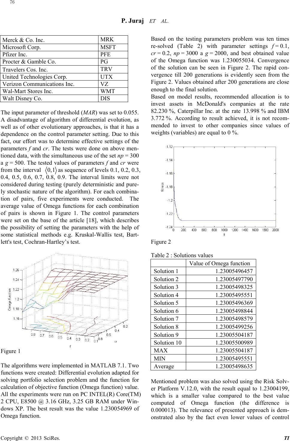

P. Juraj ET AL.

Merck & Co. Inc. M RK

Microsoft Corp. MSFT

Pfizer Inc. PFE

Procter & Gamble Co. PG

Travelers Cos. Inc. TRV

United Technologies Corp. UTX

Verizon Communications Inc. VZ

Wal-Mart Stores Inc. WMT

Walt Disney Co. DIS

The input parameter of threshold (MAR) was set to 0.055.

A disadvantage of algorithm of differential evolution, as

well as of other evolutionary approaches, is that it has a

dependence on the control parameter setting. Due to this

fact, our effort was to determine effective settings of the

parameters f and cr. The tests were done on above men-

tioned data, with the simultaneous use of the set np = 300

a g = 500. The tested values of parameters f and cr were

from the interval

0,1

as sequence of levels 0.1, 0.2, 0.3,

0.4, 0.5, 0.6, 0.7, 0.8, 0.9. The interval limits were not

considered during testing (purely deterministic and pure-

ly stochastic nature of the algorithm). For each combina-

tion of pairs, five exp er imen ts were conducted. The

average value of Omega functions for each combination

of pairs is shown in Figure 1. The control parameters

were set on the base of the article [18], which describes

the possibility of setting the parameters with the help of

some statistical methods e.g. Kr uskal-Wallis test, Bart-

lett's test, Cochran-Hartley’s test.

Figure 1

The algorithms were implemented in MATLAB 7.1. Two

functions were created: Differential evolution adapted for

solving portfolio selection problem and the function for

calculation of objective function (Omega function) value.

All the experiments were run on PC INTEL(R) Core(TM)

2 CPU, E8500 @ 3.16 GHz, 3.25 GB RAM under Win-

dows XP. The best result was the value 1.230054969 of

O mega function.

Based on the testing parameters problem was ten times

re-solved (Table 2) wi th parameter settin gs f = 0.1,

cr = 0.2, np = 3000 a g = 2000, and best obtained value

of the Omega function was 1.230055034. Convergence

of the solution can be seen in Figure 2. The rapid con-

vergence till 200 generations is evidently seen from the

Figure 2. Values obtained afte r 200 generations are close

enou gh to the final solution.

Based on model results, recommended allocation is to

inves t assets in McDonald's companies at the rate

82.230 %, Caterpillar Inc. at the rate 13.998 % and IBM

3.772 %. According to result achieved, it is not recom-

mended to invest to other companies since values of

weights (variables) are equal to 0 %.

Figure 2

Table 2 : Solutions values

Value of Omega function

Solution 1 1.23005496457

Solution 2 1.23005497790

Solution 3 1.23005498325

Solution 4 1.23005495551

Solution 5 1.23005496369

Solution 6 1.23005498844

Solution 7 1.23005498579

Solution 8 1.23005499256

Solution 9 1.23005504187

Solution 10 1.23005500989

MAX 1.23005504187

MIN 1.23005495551

Avera ge 1.23005498635

Mentioned problem was also solved using the Risk Solv-

er Platform V.12.0, with the result equal to 1.23004199,

which is a smaller value compared to the best value

computed of Omega function (the difference is

0.000013). The relevance of presented approach is dem-

onstrated also by the fact even lower values of control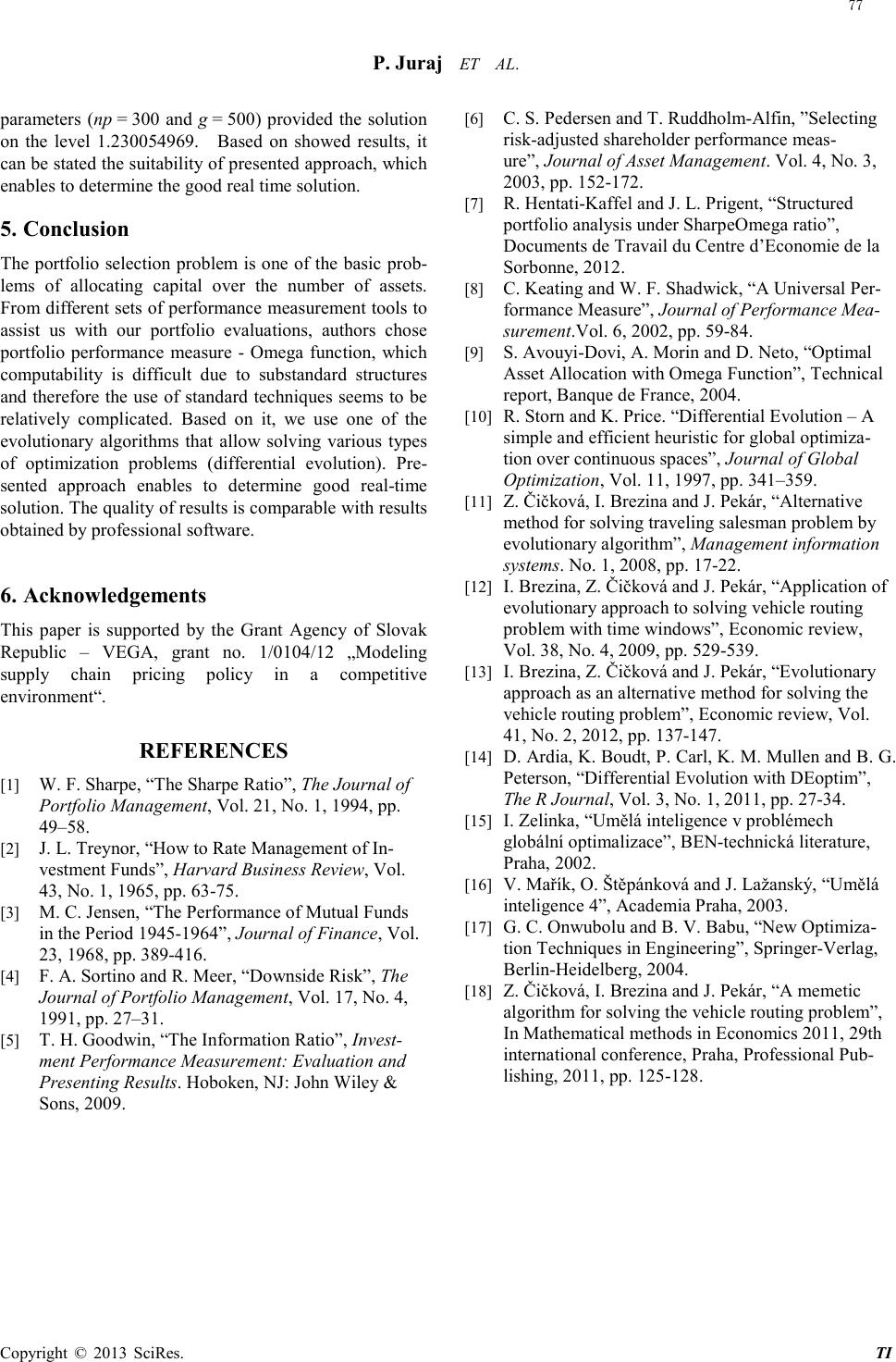

P. Juraj ET AL.

parameters (np = 300 and g = 500) provided the solution

on the level 1.230054969. Based on showed resul ts, it

can be stated the suitability of presented approach, which

enables to determine the good real time solution.

5. Conclusion

The portfolio selection problem is one of the basic prob-

lems of allocating capital over the number of assets.

Fro m differ ent sets of performance measurement tools to

assist us with our portfolio evaluations, authors chose

portfolio performance measure - Omega function, which

computability is difficult due to substandard structures

and therefore the use of standard techniques seems to be

relatively complicated. Based on it, we use one of the

evolutionary algorithms that allow solving various types

of optimization problems (differential evolution). Pre-

sented approach enables to determine good real-time

solution. The quality of results is comparable with results

obtained by professional software.

6. Acknowledgements

This paper is supported by the Grant Agency of Slovak

Republic – VEGA, grant no. 1/0104/12 „Modeling

supply chain pricing policy in a competitive

environ ment“.

REFERENCES

[1] W. F. Sharp e , “The Sharpe Ratio”, The Journal of

Portfolio Management, Vol . 21, No. 1, 1994, pp.

49–58.

[2] J. L. Treyno r , “How to Rate Management of In-

vestment Funds”, Harvard Business Review, Vol.

43, No. 1, 1965, pp. 63-75.

[3] M. C. Jensen, “The Performance of Mutual Funds

in the Period 1945-1964”, Journal of Finance, Vol.

23, 1968, pp. 389-416.

[4] F. A. Sortino and R. Meer, “Downside Risk”, The

Journal of Portfolio Management, Vol. 17, No. 4,

1991, pp. 27–31.

[5] T. H. Goodwin, “The Information Ratio”, Invest-

ment Performance Measurement: Evaluation and

Presenting Results. Hoboken, NJ: John Wiley &

Sons, 2009.

[6] C. S. Pedersen and T. Ruddholm-Alfin, ”Selecting

risk-adjusted shareholder performance meas-

ure”, Journal of Asset Management. Vol. 4, No. 3,

2003, pp. 152-172.

[7] R. Hentati-Kaffe l and J. L. Prigent , “Structured

portfolio analysis under SharpeOmega ratio”,

Documents de Travail du Centre d’Economie de la

Sorbonne, 2012.

[8] C. Keating and W. F. Shadwick, “A Universal Per-

formance Measure”, Journal of Performance Mea-

sureme nt .Vol. 6, 2002, pp. 59-84.

[9] S. Avouyi-Dovi, A. Morin and D. Neto, “Optimal

Asset Allocation with Omega Function”, Technical

report, Banque de France, 2004.

[10] R. Storn and K. Price. “Differential Evolution – A

simple and efficient heuristic for global optimiza-

tion over continuous spaces”, Journal of Global

Optimization , Vol. 11, 1997, pp. 341–359.

[11] Z. Čičková, I. Brezina and J. Pekár, “Alternative

method for solving traveling salesman problem by

evolutionary algorithm”, Management information

system s. No. 1, 2008, pp. 17-22.

[12] I. Brezina, Z. Či čková a nd J. Pekár, “Application of

evolutionary approach to solving vehicle routing

problem with time windows”, Economic review,

Vol. 38, No. 4, 2009, pp. 529-539.

[13] I. Brezina, Z. Čičko vá a nd J. Pekár, “Evolutionary

approach as an alternative method for solving the

vehicle routing problem”, Economic review, Vo l.

41, No. 2, 2012, pp. 137-147.

[14] D. Ardia, K. Boudt, P. Carl, K. M. Mullen and B. G.

Peterson, “Differential Evolution with DEoptim”,

The R Journal, Vol. 3, No. 1, 2011, pp. 27-34.

[15] I. Zelinka, “Umělá inteligence v problémech

globální optimalizace”, BEN-technická literature,

Pr aha , 2002.

[16] V. Mařík, O. Štěpánková and J. Lažanský, “Umělá

inteligence 4”, Academia Praha, 2003.

[17] G. C. Onwubolu and B. V. Babu, “New Optimiza-

tion Techniques in Engineering”, Springer-Verlag,

Berlin-Heidelberg, 2004.

[18] Z. Čičková, I. Brezina and J. Pekár, “A memetic

algorithm for solving the vehicle routing problem”,

In Mathematical methods in Economics 2011, 29th

international conference, Praha, Professional Pub-

lishing, 2011, pp. 125-128.