

Paper Menu >>
Journal Menu >>
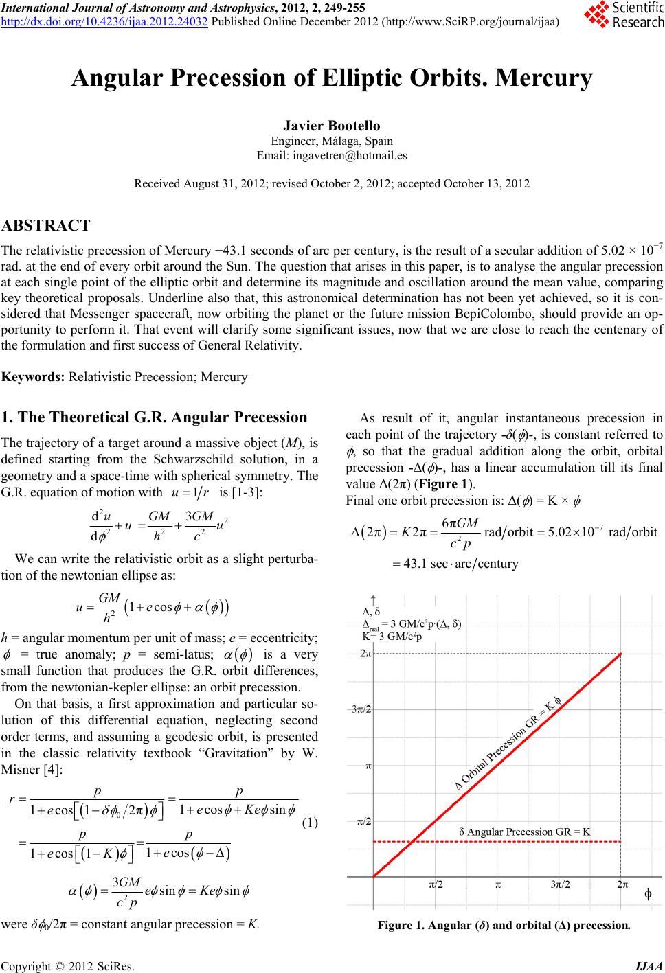 International Journal of Astronomy and Astrophysics, 2012, 2, 249-255 http://dx.doi.org/10.4236/ijaa.2012.24032 Published Online December 2012 (http://www.SciRP.org/journal/ijaa) Angular Precession of Elliptic Orbits. Mercury Javier Bootello Engineer, Málaga, Spain Email: [email protected] Received August 31, 2012; revised October 2, 2012; accepted October 13, 2012 ABSTRACT The relativistic precession of Mercury −43.1 seconds of arc per century, is the result of a secular addition of 5.02 × 10⁻⁷ rad. at the end of every orbit around the Sun. The question that arises in this paper, is to analyse the angular precession at each single point of the elliptic orbit and determine its magnitude and oscillation around the mean value, comparing key theoretical proposals. Underline also that, this astronomical determination has not been yet achieved, so it is con- sidered that Messenger spacecraft, now orbiting the planet or the future mission BepiColombo, should provide an op- portunity to perform it. That event will clarify some significant issues, now that we are close to reach the centenary of the formulation and first success of General Relativity. Keywords: Relativistic Precession; Mercury 1. The Theoretical G.R. Angular Precession The trajectory of a target around a massive object (M), is defined starting from the Schwarzschild solution, in a geometry and a space-time with spherical symmetry. The G.R. equation of motion with 1ur is [1-3]: 2 2 222 d3 d uGMGM uu hc We can write the relativistic orbit as a slight perturba- tion of the newtonian ellipse as: 21cos GM ue h h = angular momentum per unit of mass; e = eccentricity; = true anomaly; p = semi-latus; is a very small function that produces the G.R. orbit differences, from the newtonian-kepler ellipse: an orbit precession. On that basis, a first approximation and particular so- lution of this differential equation, neglecting second order terms, and assuming a geodesic orbit, is presented in the classic relativity textbook “Gravitation” by W. Misner [4]: 01cos sin 1cos1 2π 1cos 1cos1 pp reKe e pp e eK (1) 2 3sin sin GM eKe cp were δ 0/2π = constant angular precession = K. As result of it, angular instantaneous precession in each point of the trajectory -δ( )-, is constant referred to , so that the gradual addition along the orbit, orbital precession -Δ( )-, has a linear accumulation till its final value Δ(2π) (Figure 1). Final one orbit precession is: Δ( ) = K × 7 2 6π 2π2πrad orbit5.0210rad orbit 43.1 secarccentury GM Kcp Figure 1. Angular (δ) and orbital (Δ) precession. C opyright © 2012 SciRes. IJAA 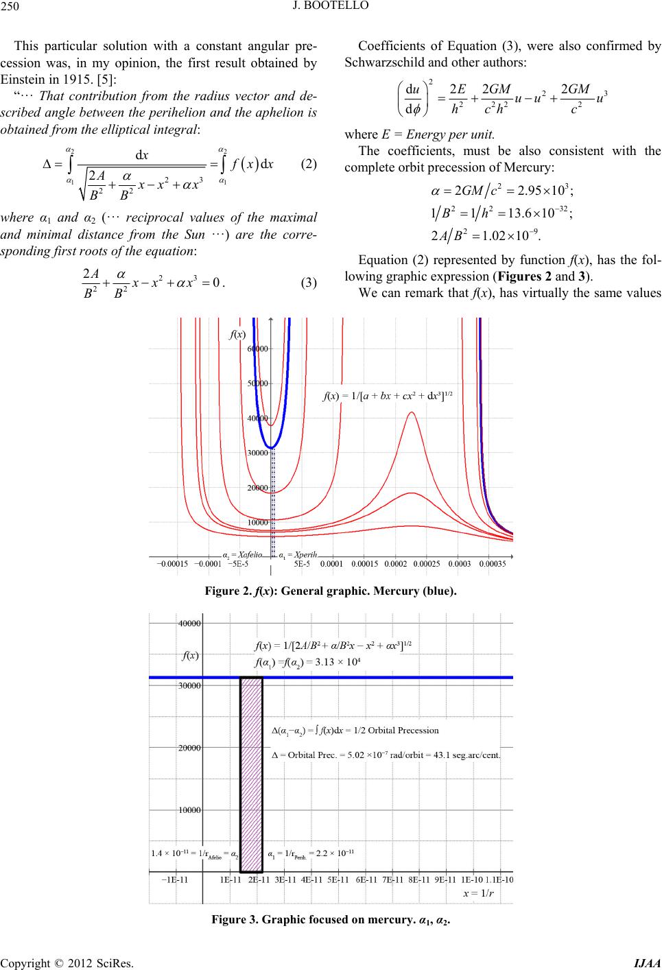 J. BOOTELLO 250 This particular solution with a constant angular pre- cession was, in my opinion, the first result obtained by Einstein in 1915. [5]: “··· That contribution from the radius vector and de- scribed angle between the perihelion and the aphelion is obtained from the elliptical integral: 2 11 23 22 dd 2 x2 f xx Axx x BB (2) where α1 and α2 (··· reciprocal values of the maximal and minimal distance from the Sun ···) are the corre- sponding first roots of the equation: 23 22 20 Axx x BB . (3) Coefficients of Equation (3), were also confirmed by Schwarzschild and other authors: 2 23 222 2 d22 2 d uE GMGM uu u hchc where E = Energy per unit. The coefficients, must be also consistent with the complete orbit precession of Mercury: 23 22 3 29 22.95 1113.610 21.0210. GM c Bh AB 2 10; ; Equation (2) represented by function f(x), has the fol- lowing graphic expression (Figures 2 and 3). We can remark that f(x), has virtually the same values Figure 2. f(x): General graphic. Mercury (blue). Figure 3. Graphic focused on mercury. α1, α2. Copyright © 2012 SciRes. IJAA 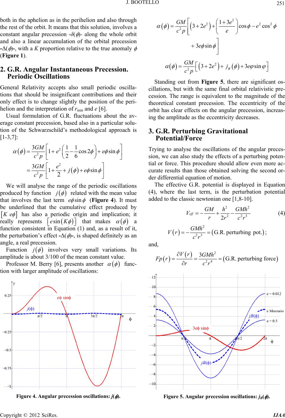 J. BOOTELLO 251 both in the aphelion as in the perihelion and also through the rest of the orbit. It means that this solution, involves a constant angular precession -δ( )- along the whole orbit and also a linear accumulation of the orbital precession -Δ( )-, with a K proportion relative to the true anomaly (Figure 1). 2. G.R. Angular Instantaneous Precession. Periodic Oscillations General Relativity accepts also small periodic oscilla- tions that should be insignificant contributions and their only effect is to change slightly the position of the peri- helion and the interpretation of rmin and e [6]. Usual formulation of G.R. fluctuations about the av- erage constant precession, based also in a particular solu- tion of the Schwarzschild’s methodological approach is [1-3,7]: 2 2 2 2 311 1cos2si 26 31sin 2 GM ee cp GMe je cp n We will analyse the range of the periodic oscillations produced by function j related with the mean value that involves the last term sine (Figure 4). It must be underlined that the cumulative effect produced by K e has also a periodic origin and implication; it really represents sin eK that makes a function consistent in Equation (1) and, as a result of it, the perturbation’s effect -Δ( )-, is shaped definitely as an angle, a real precession. Function j involves very small variations. Its amplitude is about 3/100 of the mean constant value. Professor M. Berry [6], presents another func- tion with larger amplitude of oscillations: Figure 4. Angular precession oscillations: j( ). 2 22 2 13 32coscos 3sin GM e ee e cp e 2 2 2323 sin B GM ej e cp Standing out from Figure 5, there are significant os- cillations, but with the same final orbital relativistic pre- cession. The range is equivalent to the magnitude of the theoretical constant precession. The eccentricity of the orbit has clear effects on the angular precession, increas- ing the amplitude as the eccentricity decreases. 3. G.R. Perturbing Gravitational Potential/Force Trying to analyse the oscillations of the angular preces- sion, we can also study the effects of a perturbing poten- tial or force. This procedure should allow even more ac- curate results than those obtained solving the second or- der differential equation of motion. The effective G.R. potential is displayed in Equation (4), where the last term, is the perturbation potential added to the classic newtonian one [1,8-10]. 22 223 2 eff GM hGMh Vrrcr (4) 2 23 G.R. perturbingpot. GMh Vr cr ; and, 2 24 3G.R.perturbing force Vr GMh Fp rrcr Figure 5. Angular precession oscillations: jB( ). Copyright © 2012 SciRes. IJAA 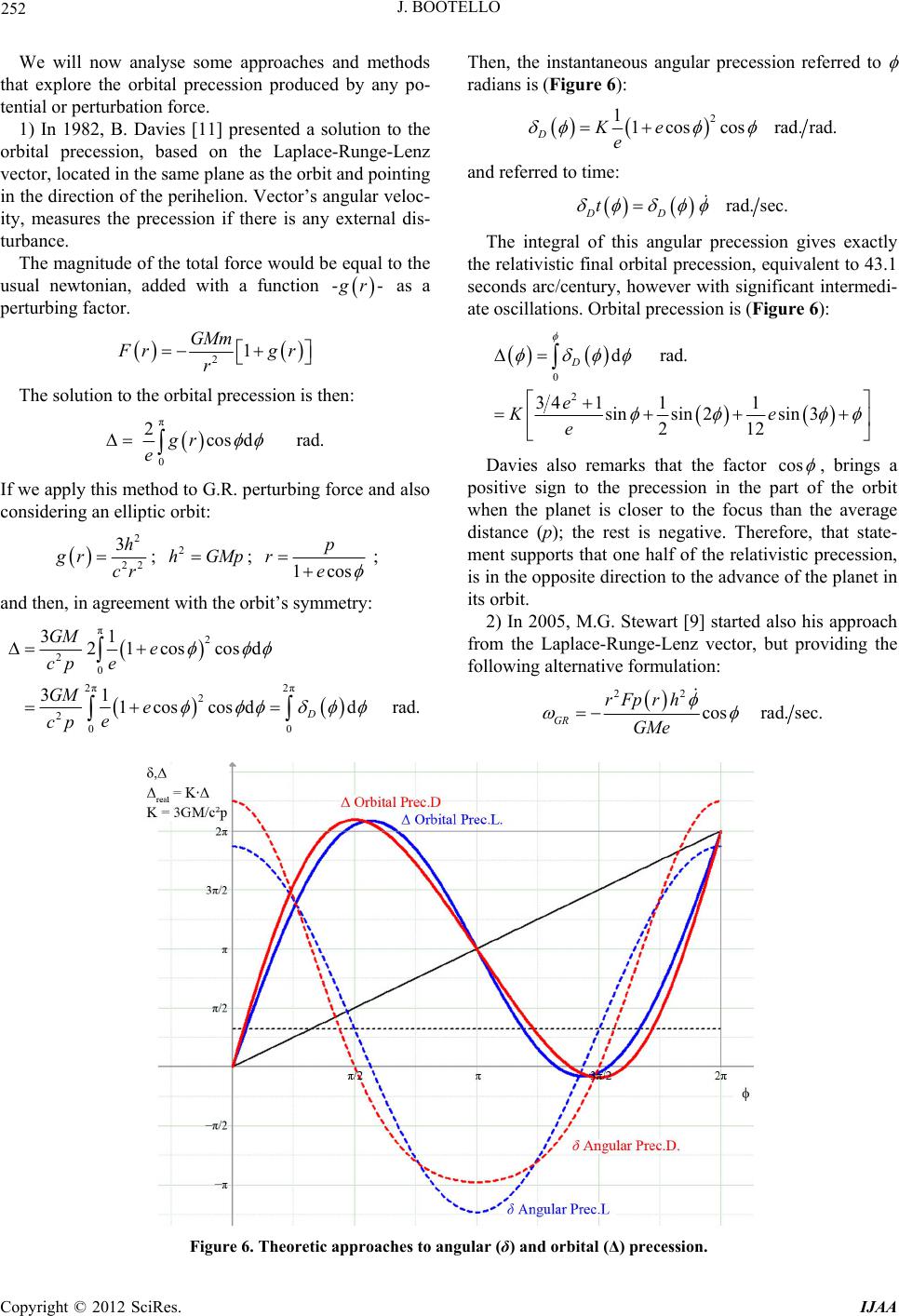 J. BOOTELLO 252 We will now analyse some approaches and methods that explore the orbital precession produced by any po- tential or perturbation force. 1) In 1982, B. Davies [11] presented a solution to the orbital precession, based on the Laplace-Runge-Lenz vector, located in the same plane as the orbit and pointing in the direction of the perihelion. Vector’s angular veloc- ity, measures the precession if there is any external dis- turbance. The magnitude of the total force would be equal to the usual newtonian, added with a function -- g r as a perturbing factor. 21 GMm F rg r r The solution to the orbital precession is then: π 0 2cosdrad.gr e If we apply this method to G.R. perturbing force and also considering an elliptic orbit: 2 22 3h gr cr ; ; 2 hGMp1cos p re ; and then, in agreement with the orbit’s symmetry: π 2 2 0 2π2π 2 2 00 31 21cos cosd 31 1coscos ddrad. D GM e e cp GM e e cp Then, the instantaneous angular precession referred to radians is (Figure 6): 2 11coscosrad. rad. DKe e and referred to time: rad. sec. DD t The integral of this angular precession gives exactly the relativistic final orbital precession, equivalent to 43.1 seconds arc/century, however with significant intermedi- ate oscillations. Orbital precession is (Figure 6): 0 2 drad. 34 111 sinsin 2sin 3 212 D e Ke e Davies also remarks that the factor cos , brings a positive sign to the precession in the part of the orbit when the planet is closer to the focus than the average distance (p); the rest is negative. Therefore, that state- ment supports that one half of the relativistic precession, is in the opposite direction to the advance of the planet in its orbit. 2) In 2005, M.G. Stewart [9] started also his approach from the Laplace-Runge-Lenz vector, but providing the following alternative formulation: 22 cosrad. sec. GR rFprh GMe Figure 6. Theoretic approaches to angular (δ) and orbital (Δ) precession. Copyright © 2012 SciRes. IJAA 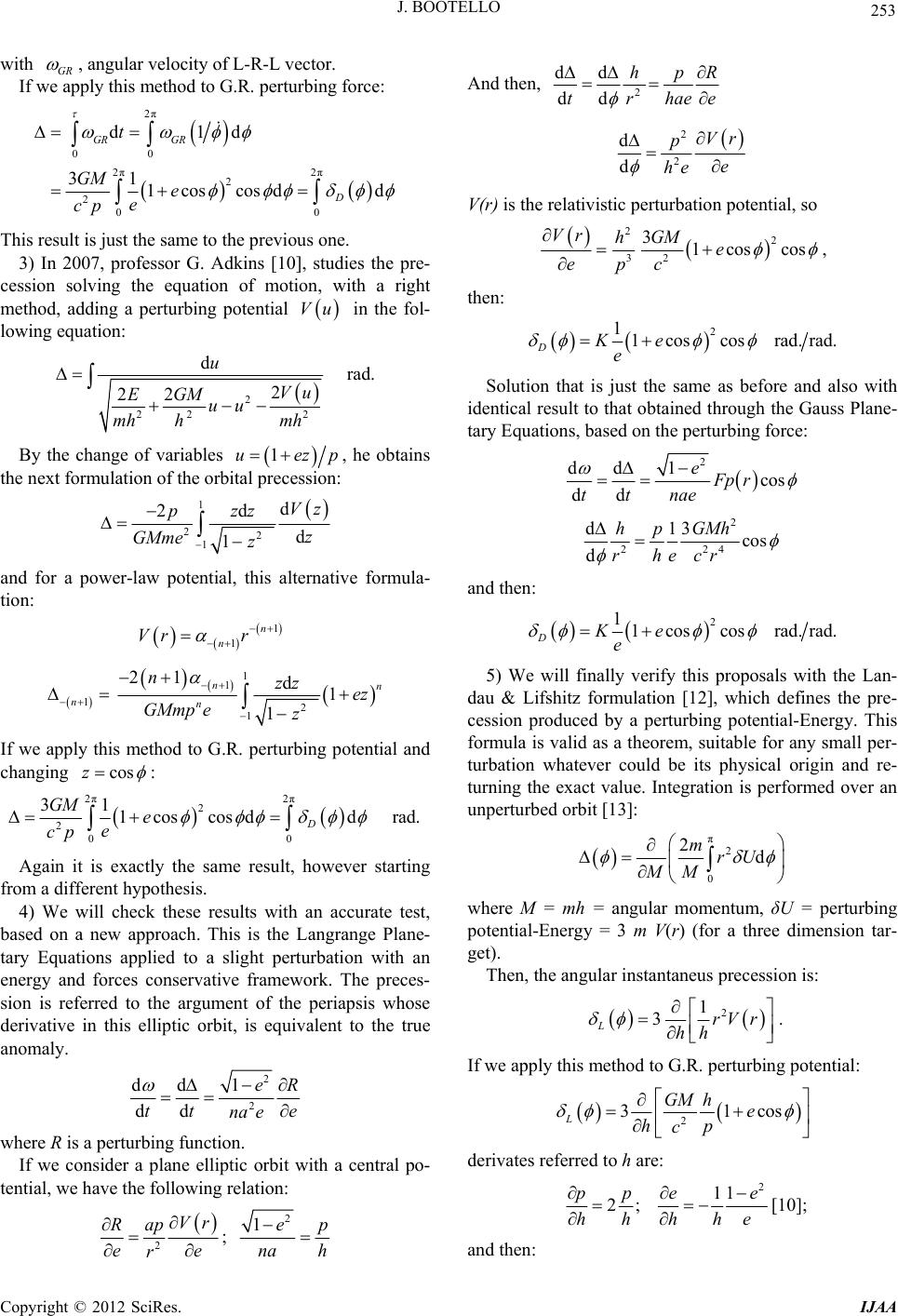 J. BOOTELLO 253 with GR , angular velocity of L-R-L vector. If we apply this method to G.R. perturbing force: 2π 00 2π2π 2 2 0 d1d 31 1cos cosdd GR GR D t GM e e cp 0 This result is just the same to the previous one. 3) In 2007, professor G. Adkins [10], studies the pre- cession solving the equation of motion, with a right method, adding a perturbing potential in the fol- lowing equation: Vu 2 22 2 drad. 2 22 u Vu EGM uu mh hmh By the change of variables 1uez p , he obtains the next formulation of the orbital precession: 1 22 1 d 2d d 1 Vz pzz z GMme z and for a power-law potential, this alternative formula- tion: 1 1 n n Vr r 1 1 12 1 21 d1 1 nn nn nzz ez GMmp ez If we apply this method to G.R. perturbing potential and changing cosz : 2π2π 2 2 00 31 1coscos ddrad. D GM e e cp Again it is exactly the same result, however starting from a different hypothesis. 4) We will check these results with an accurate test, based on a new approach. This is the Langrange Plane- tary Equations applied to a slight perturbation with an energy and forces conservative framework. The preces- sion is referred to the argument of the periapsis whose derivative in this elliptic orbit, is equivalent to the true anomaly. 2 2 dd 1 dd eR tt na e e where R is a perturbing function. If we consider a plane elliptic orbit with a central po- tential, we have the following relation: 2 Vr Rap ee r ; 2 1ep na h And then, 2 dd dd hp thae e r R 2 2 d d Vr p e he V(r) is the relativistic perturbation potential, so 22 32 31cos cos Vr hGM e epc , then: 2 11coscosrad. rad. DKe e Solution that is just the same as before and also with identical result to that obtained through the Gauss Plane- tary Equations, based on the perturbing force: 2 dd 1cos dd eFp r ttnae 2 224 d13 cos d hpGMh he rcr and then: 2 11coscosrad. rad. DKe e 5) We will finally verify this proposals with the Lan- dau & Lifshitz formulation [12], which defines the pre- cession produced by a perturbing potential-Energy. This formula is valid as a theorem, suitable for any small per- turbation whatever could be its physical origin and re- turning the exact value. Integration is performed over an unperturbed orbit [13]: π 2 0 2d mrU MM where M = mh = angular momentum, δU = perturbing potential-Energy = 3 m V(r) (for a three dimension tar- get). Then, the angular instantaneus precession is: 2 1 3 LrV r hh . If we apply this method to G.R. perturbing potential: 2 31co L GM he hp cs derivates referred to h are: 2 11 2; ppe e hhhhe [10]; and then: Copyright © 2012 SciRes. IJAA 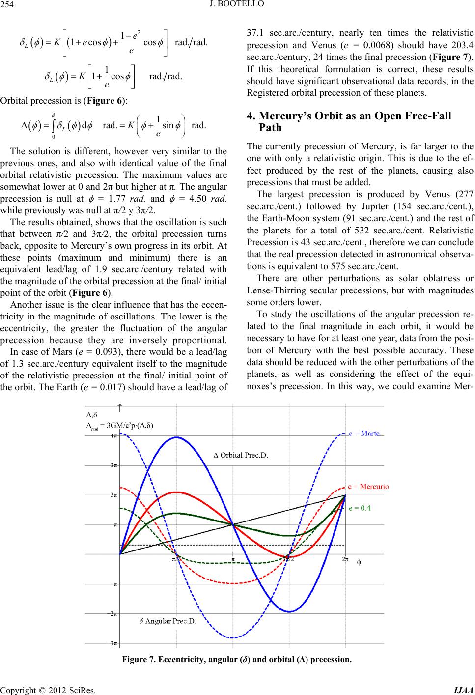 J. BOOTELLO 254 2 1 1coscosrad. rad. L e Ke e 1 1cosrad.rad. LKe Orbital precession is (Figure 6): 0 1 drad.sinrad LKe . The solution is different, however very similar to the previous ones, and also with identical value of the final orbital relativistic precession. The maximum values are somewhat lower at 0 and 2π but higher at π. The angular precession is null at = 1.77 rad. and = 4.50 rad. while previously was null at π/2 y 3π/2. The results obtained, shows that the oscillation is such that between π/2 and 3π/2, the orbital precession turns back, opposite to Mercury’s own progress in its orbit. At these points (maximum and minimum) there is an equivalent lead/lag of 1.9 sec.arc./century related with the magnitude of the orbital precession at the final/ initial point of the orbit (Figure 6). Another issue is the clear influence that has the eccen- tricity in the magnitude of oscillations. The lower is the eccentricity, the greater the fluctuation of the angular precession because they are inversely proportional. In case of Mars (e = 0.093), there would be a lead/lag of 1.3 sec.arc./century equivalent itself to the magnitude of the relativistic precession at the final/ initial point of the orbit. The Earth (e = 0.017) should have a lead/lag of 37.1 sec.arc./century, nearly ten times the relativistic precession and Venus (e = 0.0068) should have 203.4 sec.arc./century, 24 times the final precession (Figure 7). If this theoretical formulation is correct, these results should have significant observational data records, in the Registered orbital precession of these planets. 4. Mercury’s Orbit as an Open Free-Fall Path The currently precession of Mercury, is far larger to the one with only a relativistic origin. This is due to the ef- fect produced by the rest of the planets, causing also precessions that must be added. The largest precession is produced by Venus (277 sec.arc./cent.) followed by Jupiter (154 sec.arc./cent.), the Earth-Moon system (91 sec.arc./cent.) and the rest of the planets for a total of 532 sec.arc./cent. Relativistic Precession is 43 sec.arc./cent., therefore we can conclude that the real precession detected in astronomical observa- tions is equivalent to 575 sec.arc./cent. There are other perturbations as solar oblatness or Lense-Thirring secular precessions, but with magnitudes some orders lower. To study the oscillations of the angular precession re- lated to the final magnitude in each orbit, it would be necessary to have for at least one year, data from the posi- tion of Mercury with the best possible accuracy. These data should be reduced with the other perturbations of the planets, as well as considering the effect of the equi- oxes’s precession. In this way, we could examine Mer- n Figure 7. Eccentricity, angular (δ) and orbital (Δ) precession. Copyright © 2012 SciRes. IJAA 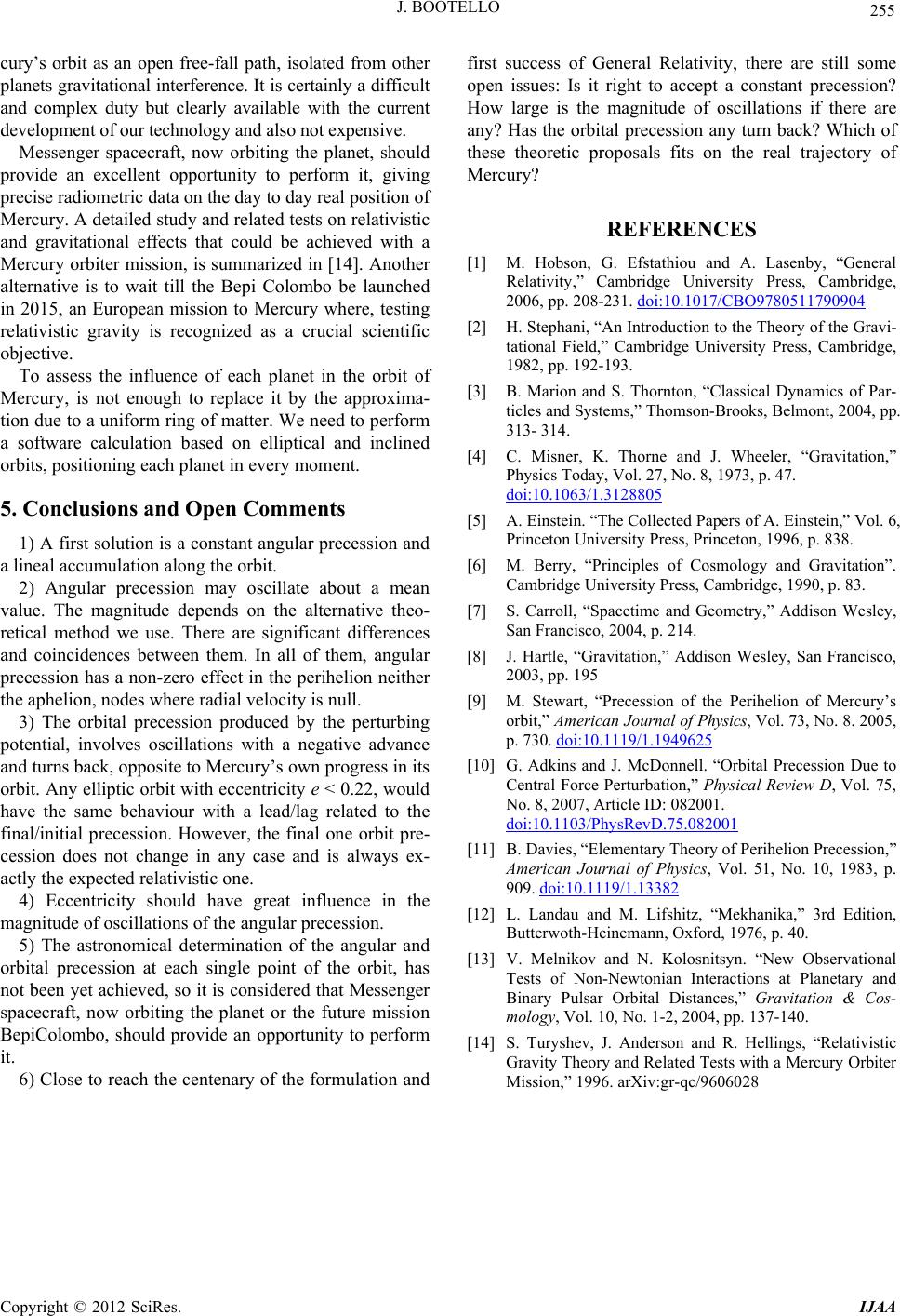 J. BOOTELLO 255 cury’s orbit as an open free-fall path, isolated from other planets gravitational interference. It is certainly a difficult and complex duty but clearly available with the current development of our technology and also not expensive. Messenger spacecraft, now orbiting the planet, should provide an excellent opportunity to perform it, giving precise radiometric data on the day to day real position of Mercury. A detailed study and related tests on relativistic and gravitational effects that could be achieved with a Mercury orbiter mission, is summarized in [14]. Another alternative is to wait till the Bepi Colombo be launched in 2015, an European mission to Mercury where, testing relativistic gravity is recognized as a crucial scientific objective. To assess the influence of each planet in the orbit of Mercury, is not enough to replace it by the approxima- tion due to a uniform ring of matter. We need to perform a software calculation based on elliptical and inclined orbits, positioning each planet in every moment. 5. Conclusions and Open Comments 1) A first solution is a constant angular precession and a lineal accumulation along the orbit. 2) Angular precession may oscillate about a mean value. The magnitude depends on the alternative theo- retical method we use. There are significant differences and coincidences between them. In all of them, angular precession has a non-zero effect in the perihelion neither the aphelion, nodes where radial velocity is null. 3) The orbital precession produced by the perturbing potential, involves oscillations with a negative advance and turns back, opposite to Mercury’s own progress in its orbit. Any elliptic orbit with eccentricity e < 0.22, would have the same behaviour with a lead/lag related to the final/initial precession. However, the final one orbit pre- cession does not change in any case and is always ex- actly the expected relativistic one. 4) Eccentricity should have great influence in the magnitude of oscillations of the angular precession. 5) The astronomical determination of the angular and orbital precession at each single point of the orbit, has not been yet achieved, so it is considered that Messenger spacecraft, now orbiting the planet or the future mission BepiColombo, should provide an opportunity to perform it. 6) Close to reach the centenary of the formulation and first success of General Relativity, there are still some open issues: Is it right to accept a constant precession? How large is the magnitude of oscillations if there are any? Has the orbital precession any turn back? Which of these theoretic proposals fits on the real trajectory of Mercury? REFERENCES [1] M. Hobson, G. Efstathiou and A. Lasenby, “General Relativity,” Cambridge University Press, Cambridge, 2006, pp. 208-231. doi:10.1017/CBO9780511790904 [2] H. Stephani, “An Introduction to the Theory of the Gravi- tational Field,” Cambridge University Press, Cambridge, 1982, pp. 192-193. [3] B. Marion and S. Thornton, “Classical Dynamics of Par- ticles and Systems,” Thomson-Brooks, Belmont, 2004, pp. 313- 314. [4] C. Misner, K. Thorne and J. Wheeler, “Gravitation,” Physics Today, Vol. 27, No. 8, 1973, p. 47. doi:10.1063/1.3128805 [5] A. Einstein. “The Collected Papers of A. Einstein,” Vol. 6, Princeton University Press, Princeton, 1996, p. 838. [6] M. Berry, “Principles of Cosmology and Gravitation”. Cambridge University Press, Cambridge, 1990, p. 83. [7] S. Carroll, “Spacetime and Geometry,” Addison Wesley, San Francisco, 2004, p. 214. [8] J. Hartle, “Gravitation,” Addison Wesley, San Francisco, 2003, pp. 195 [9] M. Stewart, “Precession of the Perihelion of Mercury’s orbit,” American Journal of Physics, Vol. 73, No. 8. 2005, p. 730. doi:10.1119/1.1949625 [10] G. Adkins and J. McDonnell. “Orbital Precession Due to Central Force Perturbation,” Physical Review D, Vol. 75, No. 8, 2007, Article ID: 082001. doi:10.1103/PhysRevD.75.082001 [11] B. Davies, “Elementary Theory of Perihelion Precession,” American Journal of Physics, Vol. 51, No. 10, 1983, p. 909. doi:10.1119/1.13382 [12] L. Landau and M. Lifshitz, “Mekhanika,” 3rd Edition, Butterwoth-Heinemann, Oxford, 1976, p. 40. [13] V. Melnikov and N. Kolosnitsyn. “New Observational Tests of Non-Newtonian Interactions at Planetary and Binary Pulsar Orbital Distances,” Gravitation & Cos- mology, Vol. 10, No. 1-2, 2004, pp. 137-140. [14] S. Turyshev, J. Anderson and R. Hellings, “Relativistic Gravity Theory and Related Tests with a Mercury Orbiter Mission,” 1996. arXiv:gr-qc/9606028 Copyright © 2012 SciRes. IJAA |