Stability Control of Stretch-Twist-Fold Flow by Using Numerical Methods

doi:10.4236/wjm.2012.26039

Paper Menu >>

Journal Menu >>

World Journal of Mechanics, 2012, 2, 334-338

doi:10.4236/wjm.2012.26039 Published Online December 2012 (http://www.SciRP.org/journal/wjm)

Stability Control of Stretch-Twist-Fold Flow by Using

Numerical Methods

Shahab Ud-Din Khan1, Yonglu Shu1, Salah Ud-Din Khan2

1Department of Mathematics and Statistics, Chongqing University, Chongqing, China

2Sustainable Energy Technologies Center, King Saud University, Riyadh, KSA

Email: [email protected]

Received September 21, 2012; revised October 24, 2012; accepted November 5, 2012

ABSTRACT

In this study, the multistep method is applied to the STF system. This method has been tested on the STF system, which

is a three-dimensional system of ODE with quadratic nonlinearities. A computer based Matlab program has been de-

veloped in order to solve the STF system. Stable and unstable position of the system has been analyzed graphically and

finally a comparison as well as accuracy between two-step sizes with detail. Newton’s method has been applied to show

the best convergence of this system.

Keywords: STF System; Chaos; Modified Method; Fixed Point Iteration Method; Newton’s Method

1. Introduction

The distinction between slow and fast dynamos was first

drawn by Vainshtein & Zeldovich (1972) in this research;

we describe the stretch-twist-fold (STF) fast dynamo,

which is the archetype of the elementary models of the

process. Basically, stretch-twist-fold is applied in fluid

mechanics in aerospace. In space, any fluid can be D-

Tracked easily so a magnetic field is required to compel

the fluid to be in the same orbit and this method is called

STF system. In this paper, we will investigate the accu-

racy of numerical method. The Multistep method was

first introduced by Goldstine, Herman H. in the begin-

ning of 1977’s. This iterative method has proven rather

successful in dealing with various scientific problems

[1-4] since it provides analytical solutions, which is a

standard numerical method. This method has also been

applied to solve nonlinear systems of ordinary differen-

tial equations. For example, H. B. Keller [5] presented an

extensive comparative study on the accuracy of the

multistep method and C. Lubich [6] studied the effects of

time steps on the stiff problem. J. O. Fatokun and I. K. O.

Ajibola [7] studied multistep method for integrating or-

dinary differential equations on manifolds. Differential

equations are used to model problems in science and en-

gineering that involve the change of some variables with

respect to another. Most of their problems require the

solution to an initial-value problem that is the solution to

a differential equation that satisfies a given initial condi-

tion. In most real-life situations the differential equation

that models the problem is too complicated to solve ex-

actly and one of two approaches is taken to approximate

the solution. The first approach is to simplify the differ-

ential equation to one that can be solved exactly and then

use the solution of the simplified equation to approxi-

mate the solution to the original equation. The other ap-

proach, which we will examine in this paper, uses meth-

ods for approximating the solution of the original prob-

lem. This is the approach that is most commonly taken,

since the approximation methods give more accurate

results and realistic error information. The objective of

this research is to solve STF system and test nonlinear

behavior with different time steps. This modified method

is able to find a stable and unstable position of STF sys-

tem. This method can also give the exact values after

iteration results. Newton’s method is able to show the

best convergence than fixed point iteration method.

2. Stretch-Twist-Fold Flow (STF)

The STF flow is defined as







222

11 33,

xtz xy

ytxy zxz

ztx yzxy













 



(1)

where α = 0.1, β = 1 are positive real parameters and re-

lated to the ratios of intensities of the stretch, twist and

fold ingredients of the flow.

3. Description of Methods

The methods we consider in this section do not produce

a continuous approximation to the solution of the ini-

tial-value problem. Rather, approximations are found at

S. U. D. KHAN ET AL.

335

certain specified and often equally spaced points. Some

method of interpolation is used if intermediate values are

needed. We need some definitions and results from the

theory of ordinary differential equations before consid-

ering methods for approximating the solutions to ini-

tial-value problems.

Definition 3.1: A function



xy is said to satisfy a

Lipschtiz condition in the variable y on a set





,,Dxyaxb y

If a constant 0L exists with the property that



xyf xyLyy







,,,

yxy D





This first part of this section is concerned with ap-

proximation the solution



x to a problem of the form



d,,for

xyax b

x

Subject to an initial conditions



ay

Lemma 3.1: Suppose that





xy is continuous on D

if f satisfies a Lipschitz condition on D in the variable y,

Then the initial-value problem



d,,for

xyax b

ya y











has a unique solution



x for axb.

The methods of Euler and Runge-kutta are called one-

step methods because the approximation for the mesh

point 1

x involves information from only one of the

previous mesh points i

although these methods can

use functional evaluation information at points between

and 1

x, they do not retain that information for

direct use in future approximations. All the information

used by these methods is obtained within the subinterval

over which the solution is being approximated. Since the

approximate solution is available at each of the mesh

points 01

,, ,

xx before the approximation at 1



is obtained and because the error



11ii

yyx



 tends

to increase with I, it seems reasonable to develop meth-

ods that these more accurate previous data when ap-

proximation the solution at 1



Methods using the approximation at more than one

previous mesh point to determine the approximation at

the next point are called multistep methods.

Definition 3.2: An m-step multistep method for solv-

ing the initial-value problem (3.1) is one whose differ-

ence equation for finding the approximation 1i



At the mesh point 1

x can be represented by the

following equation,

where p is an integer greater than 0



 

1011111 11

011

iimimii

iimim im

ji jij

yayayay hbfxy

bfxyb fxy

ayh bf



 







 





 







(A)

When b–1 = 0 then the method is called explicit or

open. Since Equation (A) then gives 1i

y explicitly in

terms of previously determine values. When 10b



then the method is called implicit or closed. Since 1i



occurs on both sides of Equation (A) and is specified

only implicitly.

To begin the derivation of the multistep methods, note

that the solution to the initial-value problem (3.1), if in-

tegrated over the interval





x has the property that

 



1,d

yxyxf xyxx





 (B)

Since we cannot integrate



xy x without know-

ing





x the solution to the problem, we instead inte-

grate an interpolating





Lx to



xy x that is de-

termined by some of the previously obtained data points













00 11

,,,,,,

yxy xy Equation (B) becomes



xy Lxx







3.1. Modified Method

Use the modified APC method to solve STF system. This

method is derived from ABF-Explicit m-step technique

and AM-Implicit m-step technique. The simulation done

of this paper is for the time range





0, 1t with two

time steps 0.01t



 and 0.001t



.

Represented formula:





111223344nn

yhbgbgbgbg

 





145516273nn

yhbgbgbgbg

 

where,

1234

567

55, 59,37, 9

19,5, 1.

bb b b

bbb





12132

4351

,,,

nn n

fgf gf

gfgy





 



3.2. Unstable Position

When α = 1, β = 0.1 and h = 0.01 then we can determine

the unstable position of the system that is shown in Ta-

ble 1 and easily analyzed by the Figure 1.

3.3. Stable Position

When α = 0.1, β = 1 and h = 0.001 then we can determine

the stable position of the system that is shown in Tabl e 2

and easily analyzed by the Figure 2.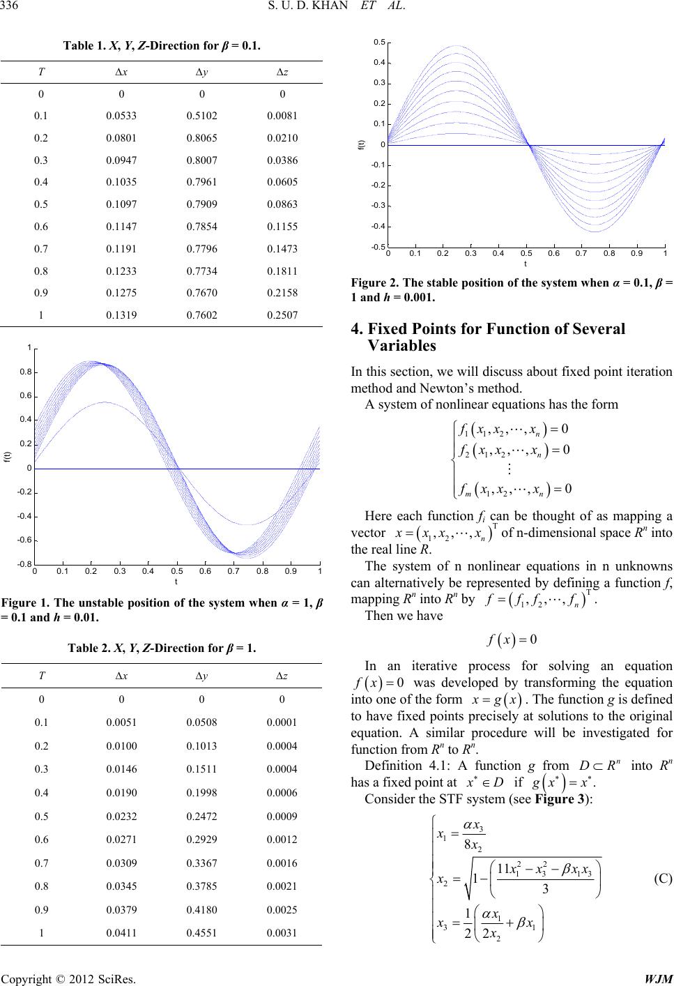

S. U. D. KHAN ET AL.

336

Table 1. X, Y, Z-Direction for β = 0.1.

T ∆x ∆y ∆z

0 0 0 0

0.1 0.0533 0.5102 0.0081

0.2 0.0801 0.8065 0.0210

0.3 0.0947 0.8007 0.0386

0.4 0.1035 0.7961 0.0605

0.5 0.1097 0.7909 0.0863

0.6 0.1147 0.7854 0.1155

0.7 0.1191 0.7796 0.1473

0.8 0.1233 0.7734 0.1811

0.9 0.1275 0.7670 0.2158

1 0.1319 0.7602 0.2507

00.1 0.20.3 0.40.5 0.6 0.70.8 0.91

-0. 8

-0. 6

-0. 4

-0. 2

0. 2

0. 4

0. 6

0. 8

f(t)

Figure 1. The unstable position of the system when α = 1, β

= 0.1 and h = 0.01.

Table 2. X, Y, Z-Direction for β = 1.

T ∆x ∆y ∆z

0 0 0 0

0.1 0.0051 0.0508 0.0001

0.2 0.0100 0.1013 0.0004

0.3 0.0146 0.1511 0.0004

0.4 0.0190 0.1998 0.0006

0.5 0.0232 0.2472 0.0009

0.6 0.0271 0.2929 0.0012

0.7 0.0309 0.3367 0.0016

0.8 0.0345 0.3785 0.0021

0.9 0.0379 0.4180 0.0025

1 0.0411 0.4551 0.0031

00.1 0.20.3 0.40.5 0.6 0.70.8 0.91

-0.5

-0.4

-0.3

-0.2

-0.1

0.1

0.2

0.3

0.4

0.5

f(t)

Figure 2. The stable position of the system when α = 0.1, β =

1 and h = 0.001.

4. Fixed Points for Function of Several

Variables

In this section, we will discuss about fixed point iteration

method and Newton’s method.

A system of nonlinear equations has the form







112

212

,,, 0

fxx x

fxxx

fxx x





















Here each function fi can be thought of as mapping a

vector



,,,

xx xof n-dimensional space Rn into

the real line R.

The system of n nonlinear equations in n unknowns

can alternatively be represented by defining a function f,

mapping Rn into Rn by



,,, .

fff f

Then we have





0fx

In an iterative process for solving an equation





0fx



was developed by transforming the equation

into one of the form





gx. The function g is defined

to have fixed points precisely at solutions to the original

equation. A similar procedure will be investigated for

function from Rn to Rn.

Definition 4.1: A function g from n

DR into Rn

has a fixed point at











Consider the STF system (see Figure 3):

13 13

xxx

































(C)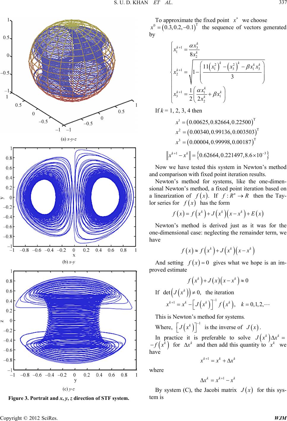

S. U. D. KHAN ET AL.

337

(a) x-y-z

(b) x-y

Figure 3. Portrait and x, y, z direction of STF system.

To approximate the fixed point

 we choose



00.3,0.2, 0.1x

the sequence of vectors generated

 

13 13

xxx





































If k = 1, 2, 3, 4 then



0.00625,0.82664,0.22500

0.00340,0.99136,0.003503

0.00004,0.99998,0.00187







0.62664,0.221497,8.6 10





Now we have tested this system in Newton’s method

and comparison with fixed point iteration results.

Newton’s method for systems, like the one-dimen-

sional Newton’s method, a fixed point iteration based on

a linearization of





x If :n

RR then the Tay-

lor series for





x has the form











 



kkk

xfx Jxxx Ex 

Newton’s method is derived just as it was for the

one-dimensional case: neglecting the remainder term, we

have









kkk

xfx Jxxx 

And setting





0fx



gives what we hope is an im-

proved estimate











fx Jxxx













det 0,



the iteration

 

1,0,1,2,

kk kk

xxJxfxk





 

 

This is Newton’s method for systems.

Where,











 is the inverse of



In practice it is preferable to solve













x for k



and then add this quantity to k

have

1kkk







where

1kk k







By system (C), the Jacobi matrix



x for this sys-

tem is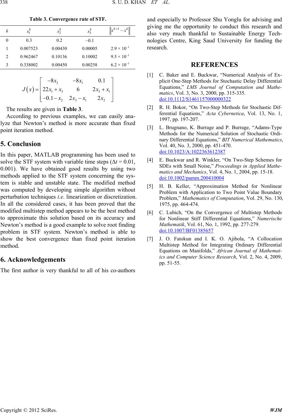

S. U. D. KHAN ET AL.

338

Table 3. Convergence rate of STF.

k 1

1kk



0 0.3 0.2 –0.1

1 0.007523 0.00430 0.00005 2.9 × 10–1

2 0.962467 0.10136 0.10002 9.5 × 10–1

3 0.338002 0.00450 0.00258 6.2 × 10–1



13 31

231 2

880.1

226 2

0.1 22

xxx xx

xxxx







 







The results are given in Table 3.

According to previous examples, we can easily ana-

lyze that Newton’s method is more accurate than fixed

point iteration method.

5. Conclusion

In this paper, MATLAB programming has been used to

solve the STF system with variable time steps (∆t = 0.01,

0.001). We have obtained good results by using two

methods applied to the STF system concerning the sys-

tem is stable and unstable state. The modified method

was computed by developing simple algorithm without

perturbation techniques i.e. linearization or discretization.

In all the considered cases, it has been proved that the

modified multistep method appears to be the best method

to approximate this solution based on its accuracy and

Newton’s method is a good example to solve root finding

problem in STF system. Newton’s method is able to

show the best convergence than fixed point iteration

method.

6. Acknowledgements

The first author is very thankful to all of his co-authors

and especially to Professor Shu Yonglu for advising and

giving me the opportunity to conduct this research and

also very much thankful to Sustainable Energy Tech-

nologies Centre, King Saud University for funding the

research.

REFERENCES

[1] C. Baker and E. Buckwar, “Numerical Analysis of Ex-

plicit One-Step Methods for Stochastic Delay Differential

Equations,” LMS Journal of Computation and Mathe-

matics, Vol. 3, No. 3, 2000, pp. 315-335.

doi:10.1112/S1461157000000322

[2] R. H. Bokor, “On Two-Step Methods for Stochastic Dif-

ferential Equations,” Acta Cybernetica, Vol. 13, No. 1,

1997, pp. 197-207.

[3] L. Brugnano, K. Burrage and P. Burrage, “Adams-Type

Methods for the Numerical Solution of Stochastic Ordi-

nary Differential Equations,” BIT Numerical Mathematics,

Vol. 40, No. 3, 2000, pp. 451-470.

doi:10.1023/A:1022363612387

[4] E. Buckwar and R. Winkler, “On Two-Step Schemes for

SDEs with Small Noise,” Proceedings in Applied Mathe-

matics and Mechanics, Vol. 4, No. 1, 2004, pp. 15-18.

doi:10.1002/pamm.200410004

[5] H. B. Keller, “Approximation Method for Nonlinear

Problem with Application to Two Point Value Boundary

Problem,” Mathematics of Computation, Vol. 29, No. 130,

1975, pp. 464-474.

[6] C. Lubich, “On the Convergence of Multistep Methods

for Nonlinear Stiff Differential Equations,” Numerische

Mathematik, Vol. 61, No. 1, 1992, pp. 277-279.

doi:10.1007/BF01385657

[7] J. O. Fatokun and I. K. O. Ajibola, “A Collocation

Multistep Method for Integrating Ordinary Differential

Equations on Manifolds,” African Journal of Mathemat-

ics and Computer Science Research, Vol. 2, No. 4, 2009,

pp. 51-55.