The Gain Distribution According to the Theoretical Structure and Decay Dynamics of Sodium like Cu

doi:10.4236/opj.2012.24045

Paper Menu >>

Journal Menu >>

Optics and Photonics Journal, 2012, 2, 358-366

http://dx.doi.org/10.4236/opj.2012.24045 Published Online December 2012 (http://www.SciRP.org/journal/opj)

The Gain Distribution According to the Theoretical

Structure and Decay Dynamics of Sodium-Like Cu

Wessameldin S. Abdelaziz1, Mai E. Ahmed2, Ali S. Khalil3,

Mohammed Alshaik Ahmed4, Tharwat M. El-Sherbini5

1National Institute of Laser Enhanced Sciences, Cairo University, Giza, Egypt

2Environmental Affairs Agency, Cairo, Egypt

3Tebin Institute for Metrological Studies, Helwan, Egypt

4Al-Azhar University, Gaza, Palastine

5Laboratory of Lasers and New Materials, Cairo University, Giza, Egypt

Email: [email protected]

Received August 31, 2012; revised September 30, 2012; accepted October 10, 2012

ABSTRACT

Level structure, oscillator strengths, transition probabilities and radiative life times are evaluated for 1s2 2s2 2p63l, 4l, 5l

(l = 0, 1, 2, 3, 4) states in sodium-like Cu18+. The calculations are carried out using COWAN code. The calculations

were made are compared with other results in literature where a good agreement is found, we also report on some un-

published energy values and oscillator strengths. Our results are used in the calculation of reduced population of 21 fine

structure levels over a wide rang of electron density values (1018 to 1020) and at various electron plasma temperature.

For those transitions with positive population inversion factor, the gain coefficients are evaluated and plotted against the

electron density.

Keywords: Level Structure; Oscillator Strengths; Sodium-Like Cu

1. Introduction

Successful results on soft X-ray amplification have been

achieved with the electron collisional excitation scheme

including neon-like and nickel-like isoelectronic se-

quences [1-3]. With the neon-like scheme, the required

pumping laser intensity increases rapidly as the wave-

length be comes shorter towards the water window spec-

tral region (4.4 - 2.3 nm) [4].

An important objective in the development of X-ray

lasers is to deliver a coherent, saturated output at wave-

lengths toward the water window [1].

Such saturated X-ray lasers are required for hologra-

phy [2] and microscopy [3], of biological specimens and

for deflectometry [4], interferometry [5], and radiogra-

phy [6] of dense plasma relevant to inertial confinement

fusion and laboratory astrophysics [5]. Sodium-like ions

have prominent emission lines in the UV and XUV spec-

trum of the sun. Highly charged sodium-like ions were

observed in several types of laboratory sources such as

high-voltage vacuum spark tokomak and laser-produced

plasmas [1].

Spectra of these ions have a simple structure (one elec-

tron outside a closed shell); the energy levels are practi-

cally free from effects of configuration mixing and

therefore they are well suited for a theoretical interpreta-

tion of line intensities and for diagnostic purposes. In

recent years, there have been extensive spectroscopic

studies, both experimental and theoretical, of sodium

isoelectronic sequence. [7] have used multi-configuration

Hartree Fock (MCHF) method and Non-Orthogonal

Spline configuration interaction (CI) method to evaluate

energy levels and oscillator strengths for Na-like ions up

to Fe XVI. [8] have used theoretical single—configure-

tion Dirac-Fock method to evaluate oscillator strengths

for E1 transitions in the sodium isoelectronic sequence

(Na I-Ca X). Large-scale calculations were undertaken

within the so-called Opacity Project (OP) [8] and, as a

result of broad international collaboration, a complete set

of oscillator strengths was produced for all optically al-

lowed transitions between states with 1≤ Z ≤ 14 as well

as Z = 16, 18, 20, and 26 in all stages of ionization.

However, relativistic effects were also neglected in OP

calculations and LS coupling was assumed. Therefore,

the OP data are available for multiples only and not for

individual fine-structure components. [9] assigned ex-

perimental wavelengths to 1086 lines which have oscil-

lator strengths calculated in OP and added 1163 lines

which have critically evaluated oscillator strengths. [10]

and from the US National Bureau of Standards (NBS)

publications [11-13]. Experimental lifetime measure-

W. S. ABDELAZIZ ET AL. 359

ments for the 4p and 5p levels and calculation of transi-

tion probabilities in Na I have been measured using

time-resolved laser induced fluorescence [14].

The purpose of this work is to present the energies of

21 fine structure levels, the Oscillator strengths, the tran-

sition probabilities between them in sodium-like Cu18+.

The atomic data thus obtained are used to calculate

reduced population of sodium-like Cu18+ excited levels

over a wide range of electron density and at various elec-

trons Temperatures. The gain coefficients are also calcu-

lated.

2. Computation of Atomic Structures

2.1. Model of Central Force Field

In quantum mechanics, various physical processes can be

summed by Schrödinger equation, i.e.

iii

HE (1)

In the non-relativistic case (the influence of relativistic

effect will be discussed later), the Hamiltonian of an

atomic system with N electrons is:



2π.

kine nuce e

HH HH





 







(2)

Here Hkin, He-nuc and He-e refer, respectively, to the ki-

netic energy of electrons, the Coulomb potential and the

energy of electrostatic interaction of electrons, ri is the

distance between the i-th electron and nucleus, and

iji j

rrr.

By substituting the Hamiltonian into Schrödinger

equation and solving the equation in the case of multiple

electrons and multiple energy levels, the wave function is

obtained. Now, due to the appearance of the term of in-

teraction of electrons, an exact solution cannot be ob-

tained. On the other hand, the interaction term is compa-

rable with the Coulomb potential term, so it can by no

means be ignored. An approximate solution is to adopt

the method of central force field. If it is assumed that

every electron moves in the central force field of the nu-

cleus and also in the mean force field produced by other

electrons, then we have the following effective Hamilto-

nian:



eff effeff

pZe





 





 r





(3)

2.2. Method of Calculation

The key problem in the application of central field is to

find an adequate potential function Veff. For this, in recent

decades many effective method of calculation have been

developed. Among them the more important ones are the

potential model, Hartree-Fock theory, the semi-empirical

methods. In the following we present a brief introduction

of semi-empirical methods.

Semi-empirical methods try to calculate atomic struc-

tures via solving the simplified form of the Hartree-Fock

equation. The most typical is the Hartree-Fock-Slater

method.

Afterwards, Cowan et al. revised this method and de-

veloped the RCN/RCG program used in our work. The

merit of the program is its extreme effectiveness, and the

shortcoming is its inability to estimate the precision.

2.3. Configuration Interaction

In the above-stated model of central force field, every

electron can be described with a simple wave function.

The overall wave function of atoms may be expressed

with the following Slater determinant:







11 1





 















 







 



(4)

In reality, such a description is not very precise. The

best wave function should be a linear combination of

wave functions with single configurations, and these

wave functions possess the same total angular momen-

tum and spin symmetry. This method is called the inter-

action of configurations. In the computation of atomic

structures, consideration of the configuration interaction

is the basis requirement for a program.

2.4. Relativistic Correction

In a non-relativistic system, the oscillator strengths and

dipole transitions under LS-coupling can be calculated.

In calculating forbidden transitions, jj-coupling must be

used, and for this relativistic effects have to be taken into

account. Generally speaking, the effects may be treated

in two ways. One is inclusion of Breit-Pauli operator in

the non-relativistic equation, and other is direct solution

of the Dirac equation. For the former, a mass velocity

term, the Darwin term caused by the electric moments of

electrons and the spin-orbit term are added to the Hamil-

tonian of the model of central force field [15]. For rela-

tivistic correction, the program RCN/RCG restore to the

Breit-Pauli correction.

2.5. Weighted Oscillator Strengths and Lifetimes

The oscillator strength f(γγʹ) is a physical quantity related

to line intensity I and transition probability W(γγʹ), as

given by Sobelman [16]:



2we







(5)

W. S. ABDELAZIZ ET AL.

360

with,

 

gWg fgf



.

Here m = electron mass, e = electron charge, I = is ini-

tial quantum state,



WE E



 , E(γ) initial

state energy, g = (2J + 1) is the number of degenerate

quantum state with angular momentum J (in the formula

for initial state). Quantities with primes refer to the final

state.

In the above equation, the weighted oscillator strength,

gf, is given by Cowan [17]:

8π

mca



 (6)

where g is the statistical weight of lower level, f is the

absorption oscillator strength,









EE h



 c,

h is Planck’s constant, c = light velocity, and a0 is Bohr

radius, and the electric dipole line strength is defined by:

sJPJ



 (7)

This quantity is a measure of the total strength of the

spectral line, including all possible transition between m,

m’ for different Jz Eigen states. The tensor operator P1

(first order) in the reduced matrix element is the classical

dipole moment for the atom in units of ea0.

To obtain gf, we need to calculate S first, (or its square

root):

121 \

PJs





 (8)

In a multi-configuration calculation we have to expand

the wave function



In terms of single configuration

wave-functions,



for both upper and lower levels:







 (9)

therefore, we can have the multi-configurationally ex-

pression for the square root of line strength:

1\12 \









 

 (10)

The probability per unit time of an atom in specific

state



to make a spontaneous transition to any state

with lower energy is







JAJJ







(11)

where





J is the Einstein spontaneous emis-

sion transition probability rate, for a transition from the

state.



to the state \\



The sum is over all state \\



with



\\ .EJ EJ





The Einstein probability rate is related to gf with the

following relation by [17]:

22 2

8πe

Agf



 (12)

Since the natural lifetime







is the inverse of

transition probability, then:







=,TJAJJ





 (13)

which is applicable to an isolated atom.

Interaction with matter or radiation will reduce the

lifetime of any state.

3. Computation of Gain Coefficient

The possibility of laser emission from plasma of ions of

various members of Na-like Cu via electron collisional

pumping, in the XUV and soft X-ray spectral regions is

investigated at different plasma temperatures and plasma

electron densities.

The reduced population densities are calculated by

solving the coupled rate equations [18-21].

jji ejiji

ijij ij

ei iji ijiij

ij ijij

NANC C

NNC NCNA



 



























 

(14)

here Nj is the population of level j,

is the spontane-

ous decay rate from level j to level i, e

C is the electron

collisional excitation rate coefficient, and d

C is the

electron collisional de-excitation rate coefficient, which

is related to electron collisional excitation rate coefficient

by [22,23].

exp

ji ij



gEKT













(15)

where gi and gj are the statistical weights of lower and

upper levels, respectively

The population of the jth level is obtained from the

identity [19,20,24],



jit

ite

NNN





N

(16)

where

N is the total number density of all levels of the

ion under consideration, and Nt is the total number den-

sity of all ionization stage.

Since the populations calculated from Equation (14)

are normalized such that [19,20,25]











 (17)

where n is the number of all the levels of the ion under

consideration.

W. S. ABDELAZIZ ET AL. 361

Electron collisional pumping has been applied. Colli-

sion in the lasant ion plasma will transfer the pumped

quanta to other levels, and resulted in population inver-

sions then produced between the upper and lower levels.

Once a population inversion has ensured a positive

gain through F > 0 [1].

uu l

FNg g











(18)

where u

and l

are the reduced populations of the

upper level and lower level respectively. Equation (18)

has been used to calculate the gain coefficient for Dop-

pler broadening of the various transitions in the Na-like

Cu ion.

8ππ

ul u





 

 (19)

where M is the ion mass, u



 is the transition wave-

length in cm, i is the ion temperature in T

 and u, l

represent the upper and lower transition levels respec-

tively.

The gain coefficient is expressed in terms of the upper

state density (Nu). This quantity depends on how the up-

per state is populated, as well as on the density of the

initial source state. The source state is often the ground

state for a particular ion.

4. Results and Discussions

4.1. Energy Levels

Adopting the program COWAN [17], we have computed

the parameters of atomic structures of Cu XIX (Table 1).

The energy levels considered in the calculation have 21

fine structures ranging from ground state 1s2 2s2 2p6 3s to

the excited states1s2 2s2 2p6 3d, 1s2 2s2 2p6 4s, 1s2 2s2 2p6

4d, 1s2 2s2 2p6 5s, 1s2 2s2 2p6 5s, 1s2 2s2 2p6 5d, 1s2 2s2

2p6 5 g even parity levels and 1s2 2s2 2p6 3p, 1s2 2s2 2p6

4p, 1s2 2s2 2p6 4f, 1s2 2s2 2p6 5p, 1s2 2s2 2p6 5f odd parity

levels.

Table 2 presents energy levels and fine-structure split-

ting for Cu18+ also presented the energy levels calcula-

tions of (Younis et al., 2006) the present calculations

differ by less than 0.16% for most of the levels, they

have used Configuration-Interaction Code (CIV3).and

the differ from (Nist, 2009) by less than 0.14% for most

of the levels, except in some cases like the levels 2, 3, 4,

5, 9 and 10 in which the percentage difference between

our value and the last two calculations is (0.66%, 0.66%),

(–1%, 0.28%), (0.35%, 0.27%), (0.3%, 0.35%), (–0.5%,

0.12) and (–0.49%, 0.13) respectively, This mean that

our results are in a good agreement with the theoretical

and experimental value.

Table 1. Parameters (in 1000 cm–1) used in the HFR calcu-

lations for configurations of Cu18+.

Parameter Value

Eav 3s 0

Eav 3d 817.8918

ζ 3d 2.5716

Eav 4s 2538.6141

Eav 4d 2852.2149

ζ 4d 1.1058

Eav 5s 3631.0025

Eav 5d 3784.5436

ζ 5D 0.5686

Eav 5g 3826.6066

ζ 5g 0.0683

Eav 3p 355.1267

ζ 3p 23.4863

Eav 4p 2680.7844

ζ 4p 9.3163

Eav 4f 2926.6767

ζ 4f 0.2885

Eav 5P 3701.4463

ζ 5p 4.6147

Eav 5f 3822.256

ζ 5f 0.1487

4.2. Oscillator Strength and Transition

Probability

In the present work we report results of oscillator

strength and transition probabilities using the Cowan

code taking relativistic corrections into account.

Table 3 presents the wavelength, transition probability

and the values of oscillator strength with a comparison

against another published paper (Younis et al., 2006 [26])

and NIST. There was good agreement with (NIST, 2009

[27) and only small differences about (0.8%) there was

some similarities with the paper and high differences in

some values about (85%).

4.3. Radiative Lifetime

Table 4 contains the present results of radiative lifetime

for the upper and lower laser levels for the sodium-like

Cu. The present calculations predict that the lifetime of

the upper laser level must be longer than the lifetime of

lower one to ensure the fast depletion of the population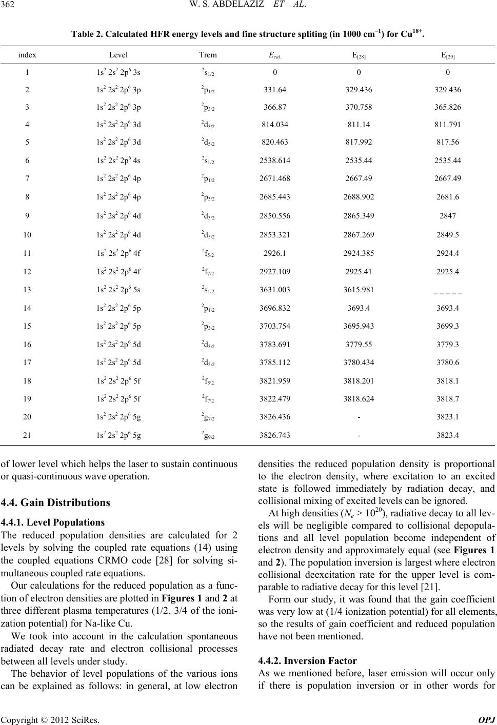

W. S. ABDELAZIZ ET AL.

362

Table 2. Calculated HFR energy levels and fine structure spliting (in 1000 cm–1) for Cu18+.

index Level Trem Ecal. E[28] E

[29]

1 1s2 2s2 2p6 3s 2s1/2 0 0 0

2 1s2 2s2 2p6 3p 2p1/2 331.64 329.436 329.436

3 1s2 2s2 2p6 3p 2p3/2 366.87 370.758 365.826

4 1s2 2s2 2p6 3d 2d3/2 814.034 811.14 811.791

5 1s2 2s2 2p6 3d 2d5\2 820.463 817.992 817.56

6 1s2 2s2 2p6 4s 2s1/2 2538.614 2535.44 2535.44

7 1s2 2s2 2p6 4p 2p1/2 2671.468 2667.49 2667.49

8 1s2 2s2 2p6 4p 2p3/2 2685.443 2688.902 2681.6

9 1s2 2s2 2p6 4d 2d3/2 2850.556 2865.349 2847

10 1s2 2s2 2p6 4d 2d5\2 2853.321 2867.269 2849.5

11 1s2 2s2 2p6 4f 2f5/2 2926.1 2924.385 2924.4

12 1s2 2s2 2p6 4f 2f7/2 2927.109 2925.41 2925.4

13 1s2 2s2 2p6 5s 2s1/2 3631.003 3615.981 _ _ _ _ _

14 1s2 2s2 2p6 5p 2p1\2 3696.832 3693.4 3693.4

15 1s2 2s2 2p6 5p 2p3\2 3703.754 3695.943 3699.3

16 1s2 2s2 2p6 5d 2d3\2 3783.691 3779.55 3779.3

17 1s2 2s2 2p6 5d 2d5\2 3785.112 3780.434 3780.6

18 1s2 2s2 2p6 5f 2f5\2 3821.959 3818.201 3818.1

19 1s2 2s2 2p6 5f 2f7\2 3822.479 3818.624 3818.7

20 1s2 2s2 2p6 5g 2g7\2 3826.436 - 3823.1

21 1s2 2s2 2p6 5g 2g9\2 3826.743 - 3823.4

of lower level which helps the laser to sustain continuous

or quasi-continuous wave operation.

4.4. Gain Distributions

4.4.1. Level Populations

The reduced population densities are calculated for 2

levels by solving the coupled rate equations (14) using

the coupled equations CRMO code [28] for solving si-

multaneous coupled rate equations.

Our calculations for the reduced population as a func-

tion of electron densities are plotted in Figures 1 and 2 at

three different plasma temperatures (1/2, 3/4 of the ioni-

zation potential) for Na-like Cu.

We took into account in the calculation spontaneous

radiated decay rate and electron collisional processes

between all levels under study.

The behavior of level populations of the various ions

can be explained as follows: in general, at low electron

densities the reduced population density is proportional

to the electron density, where excitation to an excited

state is followed immediately by radiation decay, and

collisional mixing of excited levels can be ignored.

At high densities (Ne > 1020), radiative decay to all lev-

els will be negligible compared to collisional depopula-

tions and all level population become independent of

electron density and approximately equal (see Figures 1

and 2). The population inversion is largest where electron

collisional deexcitation rate for the upper level is com-

parable to radiative decay for this level [21].

Form our study, it was found that the gain coefficient

was very low at (1/4 ionization potential) for all elements,

so the results of gain coefficient and reduced population

have not been mentioned.

4.4.2. Inversion Factor

As we mentioned before, laser emission will occur only

if there is population inversion or in other words for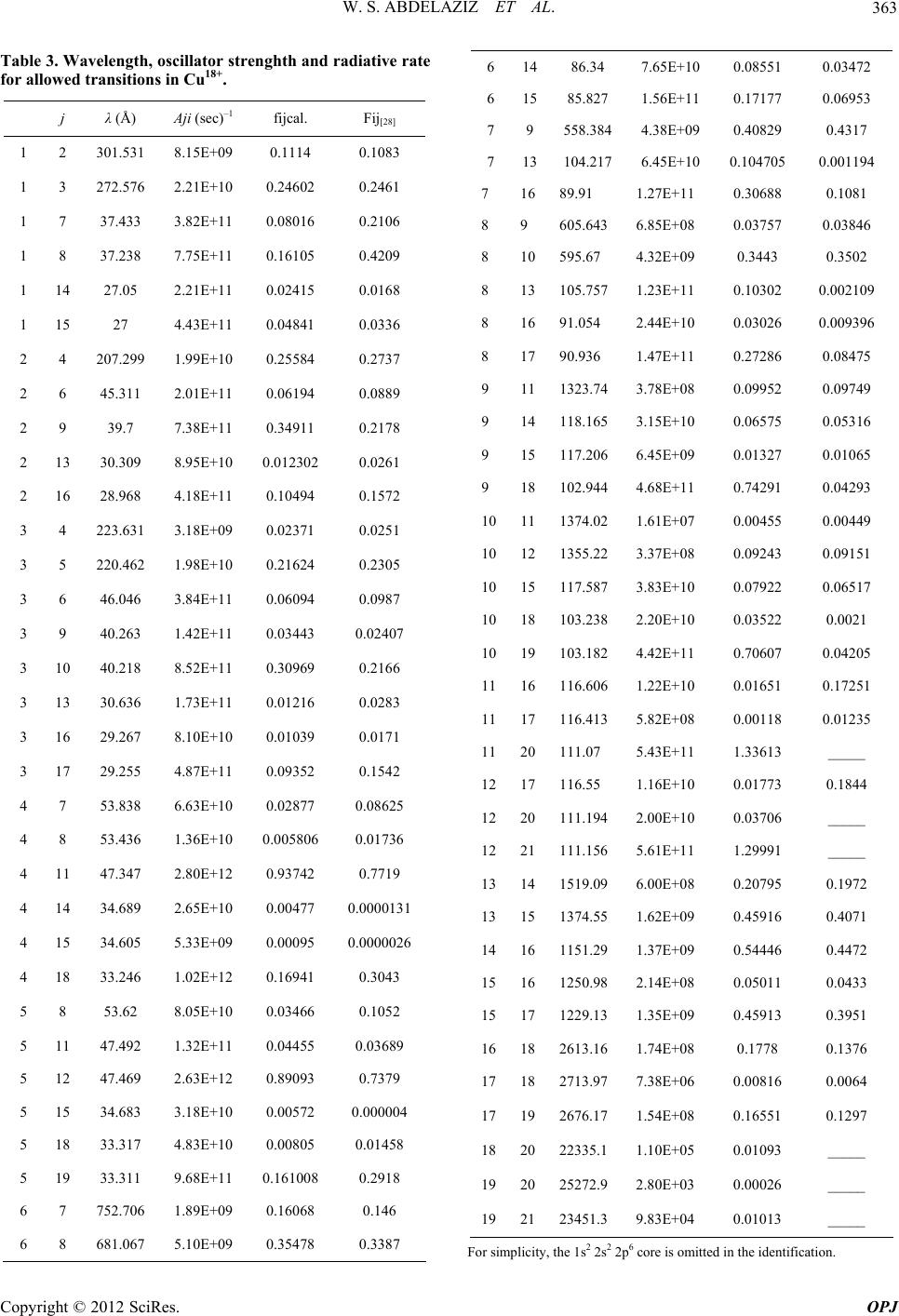

W. S. ABDELAZIZ ET AL. 363

Table 3. Wavelength, oscillator strenghth and radiative rate

for allowed transitions in Cu18+.

j λ (Å) Aji (sec)–1 fijcal. Fij[28]

1 2 301.531 8.15E+09 0.1114 0.1083

1 3 272.576 2.21E+10 0.24602 0.2461

1 7 37.433 3.82E+11 0.08016 0.2106

1 8 37.238 7.75E+11 0.16105 0.4209

1 14 27.05 2.21E+11 0.02415 0.0168

1 15 27 4.43E+11 0.04841 0.0336

2 4 207.299 1.99E+10 0.25584 0.2737

2 6 45.311 2.01E+11 0.06194 0.0889

2 9 39.7 7.38E+11 0.34911 0.2178

2 13 30.309 8.95E+10 0.012302 0.0261

2 16 28.968 4.18E+11 0.10494 0.1572

3 4 223.631 3.18E+09 0.02371 0.0251

3 5 220.462 1.98E+10 0.21624 0.2305

3 6 46.046 3.84E+11 0.06094 0.0987

3 9 40.263 1.42E+11 0.03443 0.02407

3 10 40.218 8.52E+11 0.30969 0.2166

3 13 30.636 1.73E+11 0.01216 0.0283

3 16 29.267 8.10E+10 0.01039 0.0171

3 17 29.255 4.87E+11 0.09352 0.1542

4 7 53.838 6.63E+10 0.02877 0.08625

4 8 53.436 1.36E+10 0.005806 0.01736

4 11 47.347 2.80E+12 0.93742 0.7719

4 14 34.689 2.65E+10 0.00477 0.0000131

4 15 34.605 5.33E+09 0.00095 0.0000026

4 18 33.246 1.02E+12 0.16941 0.3043

5 8 53.62 8.05E+10 0.03466 0.1052

5 11 47.492 1.32E+11 0.04455 0.03689

5 12 47.469 2.63E+12 0.89093 0.7379

5 15 34.683 3.18E+10 0.00572 0.000004

5 18 33.317 4.83E+10 0.00805 0.01458

5 19 33.311 9.68E+11 0.161008 0.2918

6 7 752.706 1.89E+09 0.16068 0.146

6 8 681.067 5.10E+09 0.35478 0.3387

6 1486.34 7.65E+10 0.08551 0.03472

6 1585.827 1.56E+11 0.17177 0.06953

7 9 558.3844.38E+09 0.40829 0.4317

7 13104.2176.45E+10 0.104705 0.001194

7 1689.91 1.27E+11 0.30688 0.1081

8 9 605.643 6.85E+08 0.03757 0.03846

8 10595.67 4.32E+09 0.3443 0.3502

8 13105.757 1.23E+11 0.10302 0.002109

8 1691.054 2.44E+10 0.03026 0.009396

8 1790.936 1.47E+11 0.27286 0.08475

9 111323.74 3.78E+08 0.09952 0.09749

9 14118.165 3.15E+10 0.06575 0.05316

9 15117.206 6.45E+09 0.01327 0.01065

9 18102.944 4.68E+11 0.74291 0.04293

10111374.02 1.61E+07 0.00455 0.00449

10121355.22 3.37E+08 0.09243 0.09151

1015117.587 3.83E+10 0.07922 0.06517

1018103.238 2.20E+10 0.03522 0.0021

1019103.182 4.42E+11 0.70607 0.04205

1116116.606 1.22E+10 0.01651 0.17251

1117116.413 5.82E+08 0.00118 0.01235

1120111.07 5.43E+11 1.33613 _____

1217116.55 1.16E+10 0.01773 0.1844

12 20 111.194 2.00E+10 0.03706 _____

1221111.156 5.61E+11 1.29991 _____

13141519.09 6.00E+08 0.20795 0.1972

13151374.55 1.62E+09 0.45916 0.4071

14161151.29 1.37E+09 0.54446 0.4472

15161250.98 2.14E+08 0.05011 0.0433

15171229.13 1.35E+09 0.45913 0.3951

16182613.16 1.74E+08 0.1778 0.1376

17182713.97 7.38E+06 0.00816 0.0064

17192676.17 1.54E+08 0.16551 0.1297

182022335.1 1.10E+05 0.01093 _____

192025272.9 2.80E+03 0.00026 _____

192123451.3 9.83E+04 0.01013 _____

For simplicity, the 1s2 2s2 2p6 core is omitted in the identification.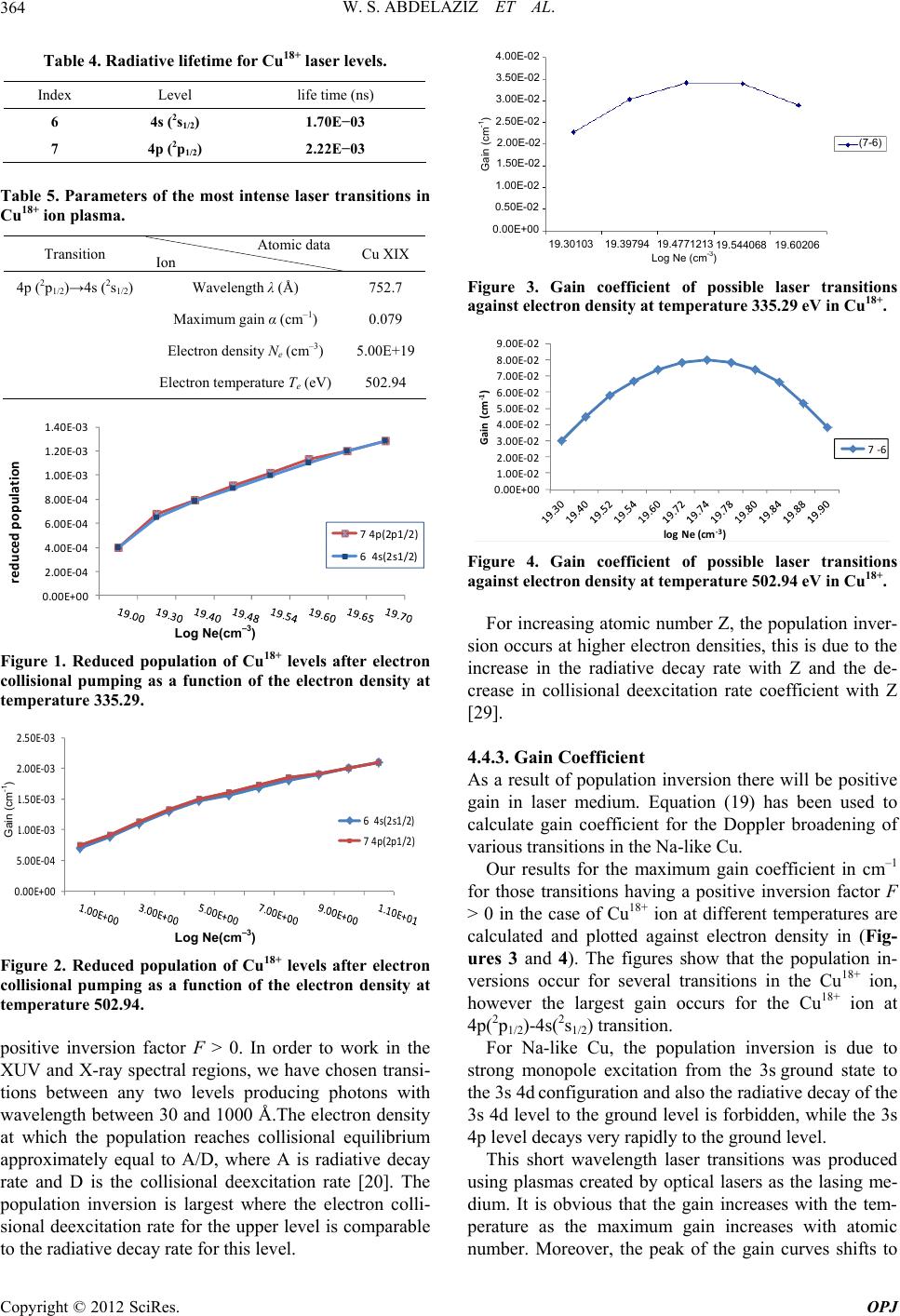

W. S. ABDELAZIZ ET AL.

364

Table 4. Radiative lifetime for Cu18+ laser levels.

Index Level life time (ns)

6 4s (2s1/2) 1.70E−03

7 4p (2p1/2) 2.22E−03

Table 5. Parameters of the most intense laser transitions in

Cu18+ ion plasma.

Transition Atomic data

Ion Cu XIX

4p (2p1/2)→4s (2s1/2) Wavelength λ (Å) 752.7

Maximum gain α (cm–1) 0.079

Electron density Ne (cm–3) 5.00E+19

Electron temperature Te (eV) 502.94

0.00E+00

2.00E-04

4.00E-04

6.00E-04

8.00E-04

1.00E-03

1.20E-03

1.40E-03

7 4p(2p1/2)

6 4s(2s1/2)

reduced population

Log Ne(cm–3)

Figure 1. Reduced population of Cu18+ levels after electron

collisional pumping as a function of the electron density at

temperature 335.29.

0.00E+00

5.00E-04

1.00E-03

1.50E-03

2.00E-03

2.50E-03

6 4s(2s1/2)

7 4p(2p1/2)

Log Ne(cm–3)

Figure 2. Reduced population of Cu18+ levels after electron

collisional pumping as a function of the electron density at

temperature 502.94.

positive inversion factor F > 0. In order to work in the

XUV and X-ray spectral regions, we have chosen transi-

tions between any two levels producing photons with

wavelength between 30 and 1000 Å.The electron density

at which the population reaches collisional equilibrium

approximately equal to A/D, where A is radiative decay

rate and D is the collisional deexcitation rate [20]. The

population inversion is largest where the electron colli-

sional deexcitation rate for the upper level is comparable

to the radiative decay rate for this level.

19.3010319.3979419.4771213 19.544068 19.60206

Log Ne (cm

)

(7-6)

4.00E-02

3.50E-02

3.00E-02

2.50E-02

2.00E-02

1.50E-02

1.00E-02

0.50E-02

0.00E+00

Gain (cm

)

Figure 3. Gain coefficient of possible laser transitions

against electron density at temperature 335.29 eV in Cu18+.

0.00E+00

1.00E-02

2.00E-02

3.00E-02

4.00E-02

5.00E-02

6.00E-02

7.00E-02

8.00E-02

9.00E-02

Gain (cm

-1

)

log Ne (cm

-3

)

7 -6

Figure 4. Gain coefficient of possible laser transitions

against electron density at temperature 502.94 eV in Cu18+.

For increasing atomic number Z, the population inver-

sion occurs at higher electron densities, this is due to the

increase in the radiative decay rate with Z and the de-

crease in collisional deexcitation rate coefficient with Z

[29].

4.4.3. Gain Coefficient

As a result of population inversion there will be positive

gain in laser medium. Equation (19) has been used to

calculate gain coefficient for the Doppler broadening of

various transitions in the Na-like Cu.

Gain (cm-

)

Our results for the maximum gain coefficient in cm–1

for those transitions having a positive inversion factor F

> 0 in the case of Cu18+ ion at different temperatures are

calculated and plotted against electron density in (Fig-

ures 3 and 4). The figures show that the population in-

versions occur for several transitions in the Cu18+ ion,

however the largest gain occurs for the Cu18+ ion at

4p(2p1/2)-4s(2s1/2) transition.

For Na-like Cu, the population inversion is due to

strong monopole excitation from the 3s ground state to

the 3s 4d configuration and also the radiative decay of the

3s 4d level to the ground level is forbidden, while the 3s

4p level decays very rapidly to the ground level.

This short wavelength laser transitions was produced

using plasmas created by optical lasers as the lasing me-

dium. It is obvious that the gain increases with the tem-

perature as the maximum gain increases with atomic

number. Moreover, the peak of the gain curves shifts to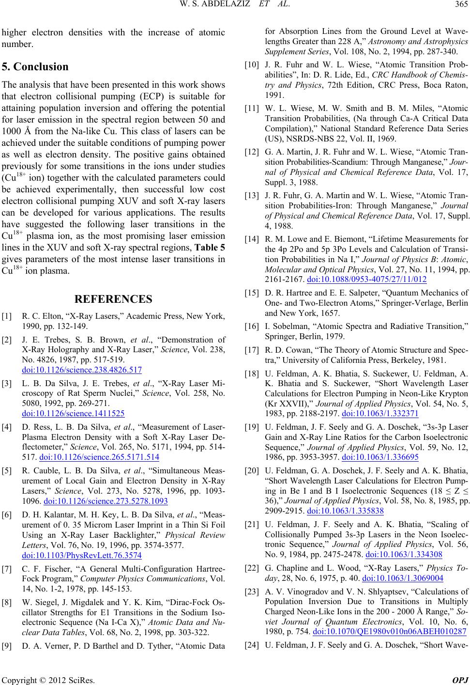

W. S. ABDELAZIZ ET AL. 365

higher electron densities with the increase of atomic

number.

5. Conclusion

The analysis that have been presented in this work shows

that electron collisional pumping (ECP) is suitable for

attaining population inversion and offering the potential

for laser emission in the spectral region between 50 and

1000 Å from the Na-like Cu. This class of lasers can be

achieved under the suitable conditions of pumping power

as well as electron density. The positive gains obtained

previously for some transitions in the ions under studies

(Cu18+ ion) together with the calculated parameters could

be achieved experimentally, then successful low cost

electron collisional pumping XUV and soft X-ray lasers

can be developed for various applications. The results

have suggested the following laser transitions in the

Cu18+ plasma ion, as the most promising laser emission

lines in the XUV and soft X-ray spectral regions, Table 5

gives parameters of the most intense laser transitions in

Cu18+ ion plasma.

REFERENCES

[1] R. C. Elton, “X-Ray Lasers,” Academic Press, New York,

1990, pp. 132-149.

[2] J. E. Trebes, S. B. Brown, et al., “Demonstration of

X-Ray Holography and X-Ray Laser,” Science, Vol. 238,

No. 4826, 1987, pp. 517-519.

doi:10.1126/science.238.4826.517

[3] L. B. Da Silva, J. E. Trebes, et al., “X-Ray Laser Mi-

croscopy of Rat Sperm Nuclei,” Science, Vol. 258, No.

5080, 1992, pp. 269-271.

doi:10.1126/science.1411525

[4] D. Ress, L. B. Da Silva, et al., “Measurement of Laser-

Plasma Electron Density with a Soft X-Ray Laser De-

flectometer,” Science, Vol. 265, No. 5171, 1994, pp. 514-

517. doi:10.1126/science.265.5171.514

[5] R. Cauble, L. B. Da Silva, et al., “Simultaneous Meas-

urement of Local Gain and Electron Density in X-Ray

Lasers,” Science, Vol. 273, No. 5278, 1996, pp. 1093-

1096. doi:10.1126/science.273.5278.1093

[6] D. H. Kalantar, M. H. Key, L. B. Da Silva, et al., “Meas-

urement of 0. 35 Microm Laser Imprint in a Thin Si Foil

Using an X-Ray Laser Backlighter,” Physical Review

Letters, Vol. 76, No. 19, 1996, pp. 3574-3577.

doi:10.1103/PhysRevLett.76.3574

[7] C. F. Fischer, “A General Multi-Configuration Hartree-

Fock Program,” Computer Physics Communications, Vol.

14, No. 1-2, 1978, pp. 145-153.

[8] W. Siegel, J. Migdalek and Y. K. Kim, “Dirac-Fock Os-

cillator Strengths for E1 Transitions in the Sodium Iso-

electronic Sequence (Na I-Ca X),” Atomic Data and Nu-

clear Data Tables, Vol. 68, No. 2, 1998, pp. 303-322.

[9] D. A. Verner, P. D Barthel and D. Tyther, “Atomic Data

for Absorption Lines from the Ground Level at Wave-

lengths Greater than 228 A,” Astronomy and Astrophysics

Supplement Series, Vol. 108, No. 2, 1994, pp. 287-340.

[10] J. R. Fuhr and W. L. Wiese, “Atomic Transition Prob-

abilities”, In: D. R. Lide, Ed., CRC Handbook of Chemis-

try and Physics, 72th Edition, CRC Press, Boca Raton,

1991.

[11] W. L. Wiese, M. W. Smith and B. M. Miles, “Atomic

Transition Probabilities, (Na through Ca-A Critical Data

Compilation),” National Standard Reference Data Series

(US), NSRDS-NBS 22, Vol. II, 1969.

[12] G. A. Martin, J. R. Fuhr and W. L. Wiese, “Atomic Tran-

sition Probabilities-Scandium: Through Manganese,” Jour-

nal of Physical and Chemical Reference Data, Vol. 17,

Suppl. 3, 1988.

[13] J. R. Fuhr, G. A. Martin and W. L. Wiese, “Atomic Tran-

sition Probabilities-Iron: Through Manganese,” Journal

of Physical and Chemical Reference Data, Vol. 17, Suppl.

4, 1988.

[14] R. M. Lowe and E. Biemont, “Lifetime Measurements for

the 4p 2Po and 5p 3Po Levels and Calculation of Transi-

tion Probabilities in Na I,” Journal of Physics B: Atomic,

Molecular and Optical Physics, Vol. 27, No. 11, 1994, pp.

2161-2167. doi:10.1088/0953-4075/27/11/012

[15] D. R. Hartree and E. E. Salpeter, “Quantum Mechanics of

One- and Two-Electron Atoms,” Springer-Verlage, Berlin

and New York, 1657.

[16] I. Sobelman, “Atomic Spectra and Radiative Transition,”

Springer, Berlin, 1979.

[17] R. D. Cowan, “The Theory of Atomic Structure and Spec-

tra,” University of California Press, Berkeley, 1981.

[18] U. Feldman, A. K. Bhatia, S. Suckewer, U. Feldman, A.

K. Bhatia and S. Suckewer, “Short Wavelength Laser

Calculations for Electron Pumping in Neon-Like Krypton

(Kr XXVII),” Journal of Applied Physics, Vol. 54, No. 5,

1983, pp. 2188-2197. doi:10.1063/1.332371

[19] U. Feldman, J. F. Seely and G. A. Doschek, “3s-3p Laser

Gain and X-Ray Line Ratios for the Carbon Isoelectronic

Sequence,” Journal of Applied Physics, Vol. 59, No. 12,

1986, pp. 3953-3957. doi:10.1063/1.336695

[20] U. Feldman, G. A. Doschek, J. F. Seely and A. K. Bhatia,

“Short Wavelength Laser Calculations for Electron Pump-

ing in Be I and B I Isoelectronic Sequences (18 ≤ Z ≤

36),” Journal of Applied Physics, Vol. 58, No. 8, 1985, pp.

2909-2915. doi:10.1063/1.335838

[21] U. Feldman, J. F. Seely and A. K. Bhatia, “Scaling of

Collisionally Pumped 3s-3p Lasers in the Neon Isoelec-

tronic Sequence,” Journal of Applied Physics, Vol. 56,

No. 9, 1984, pp. 2475-2478. doi:10.1063/1.334308

[22] G. Chapline and L. Wood, “X-Ray Lasers,” Physics To-

day, 28, No. 6, 1975, p. 40. doi:10.1063/1.3069004

[23] A. V. Vinogradov and V. N. Shlyaptsev, “Calculations of

Population Inversion Due to Transitions in Multiply

Charged Neon-Like Ions in the 200 - 2000 Å Range,” So-

viet Journal of Quantum Electronics, Vol. 10, No. 6,

1980, p. 754. doi:10.1070/QE1980v010n06ABEH010287

[24] U. Feldman, J. F. Seely and G. A. Doschek, “Short Wave-

W. S. ABDELAZIZ ET AL.

366

length Laser Calculations in the Be I, B I and C I Isoelec-

tronic Sequences,” Journal de Physique Archives, Vol. 47,

No. C6, 1986, pp. 187-202.

[25] M. J. Seaton, “Atomic Data for Opacity Calculations. I.

General Description,” Journal of Physics B: Atomic and

Molecular Physics, Vol. 20, No. 23, 1987, p. 6363.

[26] W. O Younis, S. H Allam and Th. M. El-Sherbini,

“Fine-Structure Calculations of Energy Levels, Oscillator

Strengths, and Transition Probabilities for Sodium-Like

Ions (Co XVII-Kr XXVI),” Atomic Data and Nuclear

Tables, Vol. 92, No. 2, 2005, pp. 187-205.

[27] National Institute of Standards and Technology, Physical

Reference Data, Atomic Spectra Database, Version 5, Vol.

11, 2009, pp. 3954-3958.

http://www.nist.gov/pml/data/asd.cfm

[28] S. H. Allam, “CRMO Computer Code, Private Commu-

nication,” 2003.

[29] U. Feldman, J. F. Seely and A. K. Bhatia, “Density sEN-

SITIVE X-Ray Line Ratios in the Bei, Bi, and Nei

Isoelectronic Sequences,” Journal of Applied Physics,

Vol. 58, No. 11, 1984, pp. 3954-3958.

doi:10.1063/1.335569