The Principle of Mathematical Induction Applied to the Generalized Model for the Economic Design of X-Control Charts

doi:10.4236/ojapps.2012.24035

Paper Menu >>

Journal Menu >>

Open Journal of Applied Sciences, 2012, 2, 236-240

doi:10.4236/ojapps.2012.24035 Published Online December 2012 (http://www.SciRP.org/journal/ojapps)

The Principle of Mathematical Induction Applied to the

Generalized Model for the Economic Design of

-Control Charts

Mohamed E. Seliaman1, Salih O. Duffuaa2

1Department of Information Systems, King Faisal University, Al-Ahsa, Saudi Arabia

2Department of Systems Engineering, King Fahd University of Petroleum & Minerals, Dhahran, Saudi Arabia

Email: [email protected]

Received August 4, 2012; revised September 6, 2012; accepted September 25, 2012

ABSTRACT

Rahim and Banerjee [1] developed a general model for the optimal design of

-control charts. The model minimizes

the expected cost per unit time. The heart of the model is a theorem that derives the expected total cost and the expected

cycle length. In this paper an alternative simple proof for the theorem is provided based on mathematical induction.

Keywords: Discrete Mathematics; Mathematical Induction; Statistical Quality Control; Design of

-Control Charts;

Hazard Rate Function

1. Introduction

Quality control charts are graphical statistical tools used

for process control. The first control chart was developed

by Walter A. Shewart [2]. Since then, these charts have

been widely applied in industry and also received inten-

sive attention from researchers. The

-control charts are

the most used statistical control charts when continuous

variables are used to measure quality characteristics [3].

Generally, control charts are designed using four ap-

proaches: heuristics, statistical design, economic design

and economic statistical design [4]. For more information

on the design of control charts, interested readers are re-

ferred to [1-7].

The economic design of

-control charts was origi-

nated by Duncan [8]. In his model, Duncan considers a

production process that is subject to an occurrence of an

assignable cause that will drive the process out of control.

The output of the process is measurable on a certain scale

and is normally distributed with mean 0



and standard

deviation 0



. The assignable cause is assumed to occur

according to a Possion process with intensity



and

causes a shift in the process mean to 0





, where



is a positive parameter. The control limits of the

-control chart are set at 00





, where 0



is the

standard deviation of the process. A sample of size n is

taken from the output of the process every h hour, and

used to decide whether the process is in control or not.

Banerjee and Rahim [9] generalized Duncan’s model [8]

for the economic design of

-control charts by relaxing

Duncan’s assumption that the in-control period follows an

exponential distribution. Instead, they assumed it follows

a general probability distribution having an increasing

hazard rate function. The increasing hazard rate assump-

tion resulted in the modification of the fixed sampling

interval to a variable sampling interval, dependent on the

process age. In both models, if the sample falls outside the

control limits, a search is initiated to locate the assignable

cause. If the search indicates that there is a false alarm,

the process continues. On the other hand, if the alarm is

true, repair or replacement is undertaken to bring the

process in control. Later, Rahim and Banerjee [1] ex-

tended the model in Banerjee and Rahim [9] by assuming

a general distribution of in-control periods with increasing

failure rate and considering an age-dependent repair be-

fore failure. The objective of Rahim and Banerjee’s

model [1] is to find the parameters n, hj, and k. Under the

assumptions described for this generalized model, they

derived expressions for the expected cycle length and the

total expected cost per cycle. They also presented proofs

for these expressions using a recursive argument. In this

paper a simpler and shorter mathematical induction proof

of these results is presented. Thus, our alternative proof

may make it easier for students and professors interested

in the topic within graduate coursework or further re-

search on extending the model. In this paper, we adopt the

same notations and model descriptions as defined in Ra-

him and Banerjee [1].

In order to make the paper self-contained, we describe

the main elements involved in the design of control charts,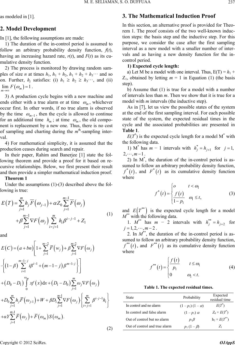

M. E. SELIAMAN, S. O. DUFFUAA 237

as modeled in [1].

2. Model Development

In [1], the following assumptions are made:

1) The duration of the in-control period is assumed to

follow an arbitrary probability density function, f(t),

having an increasing hazard rate, r(t), and F(t) as its cu-

mulative density function.

2) The process is monitored by drawing random sam-

ples of size n at times h1, h1 + h2, h1 + h2 + h3··· and so

on. Further, hj satisfies: (i) h1  h2  h3···, and (ii)



lim 1



 .

3) A production cycle begins with a new machine and

ends either with a true alarm or at time m



, whichever

occur first. In other words, if no true alarm is observed

by the time 1m



, then the cycle is allowed to continue

for an additional time m; at time m



, the old compo-

nent is replacement by a new one. Thus, there is no cost

of sampling and charting during the mth-sampling inter-

val.

4) For mathematical simplicity, it is assumed that the

production ceases during search and repair.

In their paper, Rahim and Banerjee [1] state the fol-

lowing theorem and provide a proof for it based on re-

cursive relationships. Below, we first present their result

and then provide a simpler mathematical induction proof.

Theorem 1

Under the assumptions (1)-(3) described above the fol-

lowing is true:



 



jij

EThFZ F

 

 











 



and

(1)

 

 

 



 





111

01 10

011

111

mm-

im-j

ωm

mm-m

i- j

jj-j i

jjij

jmm

ECa bnFwβFω

βiβmjβ

DD xfxxDDωFω

DhFωWβDFωβh

αYFωFωSω.





 











 























 

























(2)

3. The Mathematical Induction Proof

or Theo-

n induc-

del with one interval. Thus, E(T) = h1 +

Z1 in Equation (1) (the basis

vals less than m. Then we show that it is true for a

ach possible

ing data.

In this section, an alternative proof is provided f

rem 1. The proof consists of the two well-know

tion steps: the basis step and the inductive step. For this

purpose, we consider the case after the first sampling

interval as a new model with a smaller number of inter-

vals and as having a new density function for the in-

control period.

1) Expected cycle length:

a) Let M be a mo

, obtained by letting m = 1

ep).

b) Assume that (1) is true for a model with a number

of inter

odel with m intervals (the inductive step).

As in [7], let us view the possible states of the system

at the end of the first sampling interval. For e

ate of the system, the expected residual times in the

cycle and the associated probabilities are presented in

Table 1.

E(T*) is the expected cycle length for a model M* with

the follow

1) M* has m − 1 intervals with *



 for 1,j



2, ,1m



.

2) In M*, the duration of the in-coeriod is as-

oll

ntrol p

sumed to fow an arbitrary probability density function,





t, and





t as its cumulative density function

where

 

ft ft t











(3)

and









with th

is the expected cycle length for a model

M** e following data.

M** h1. as m − 2 intervals with **



 for

1, 2,,2jm



.

2. In M**, the duration of the in-contro as-l period is

sumed to follow an arbitrary probability density function,





t, and





t as its cumulative density function

where







ft t

ft p













(4)

Table 1. The expected residual times.

State Probability

dual time



Expected

resi

In control and no alarm (1) – p1) (1 –



E(T*)

In control and false alarm (1 – p)



arm h)



Z0 + E(T*)

Out of control but no al1

p1 (1 –



)

+ E(T**

Out of control and true alar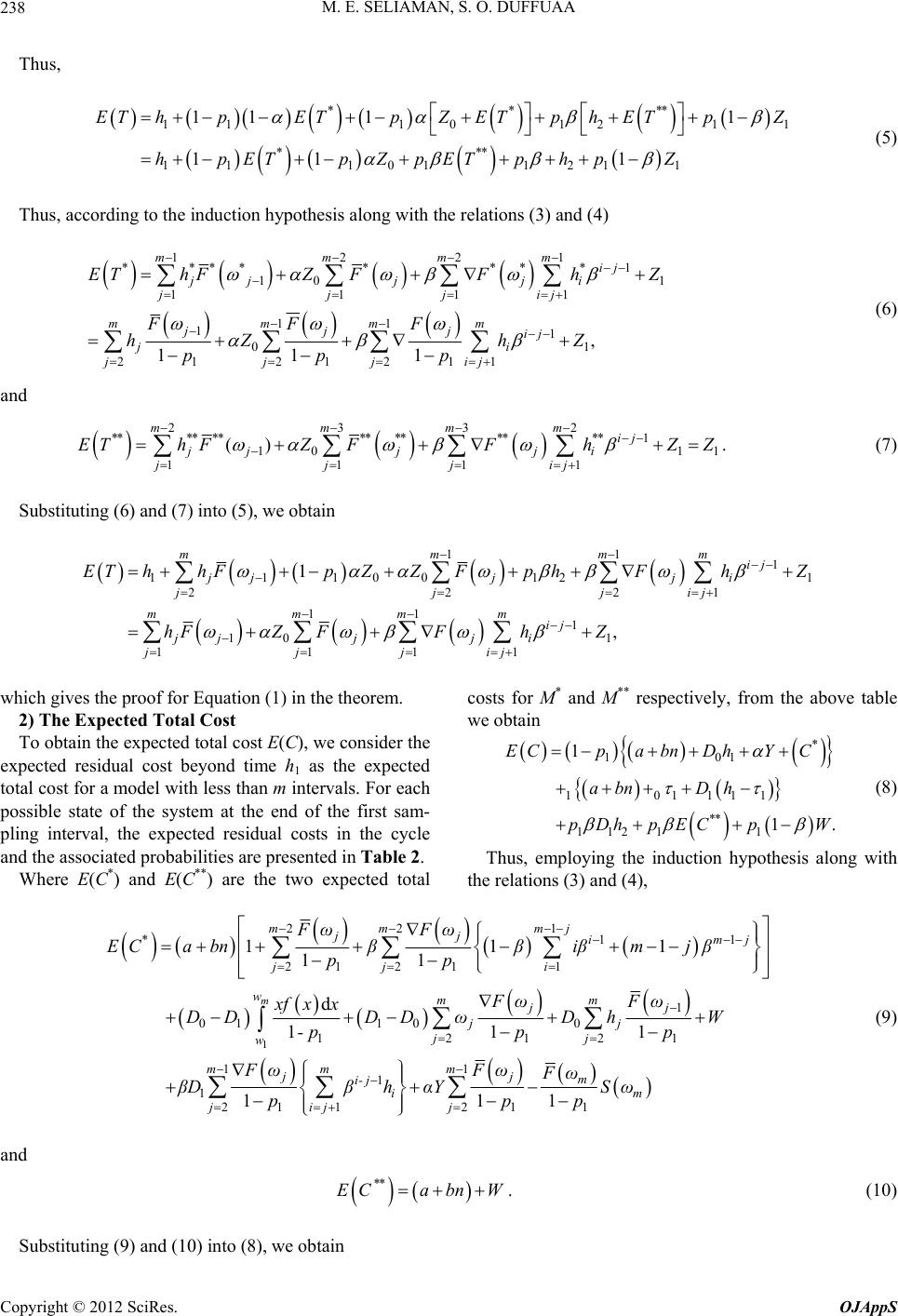

M. E. SELIAMAN, S. O. DUFFUAA

238

Thus,

 













****

1110 121

***

11101121 1

11 11

11 1

EThpETpZETph ETpZ

hpETpZpETphp Z

 

 



 



 



(5)

Thus, according to the induction hypothesis along with the relations (3) and (4)

 



  

1221mmmm

**** ****1

10 1

1111

2221

111

jj j ji

jjjij

mmmm

jjj

jjjij

EThFZ FFhZ

FFF

hZ hZ

ppp

 



 















 





(6)

and

 



2332

**** **********1

10 1

1111

()

mmmm

jjj ji

jjjij

EThFZFFhZZ

 









 



. (7)

Substituting (6) and (7) into (5), we obtain



 

  

1110012

222

11 1

10 1

1111

mmm

jjjj i

jjjij

mmmm

jjjj i

jjjij

EThhFpZZFp hFhZ

hFZFFhZ



 







 





 

 



hich gives the proof for Equation (1) in the theorem.

costs for M* and M** respectively, from the above table

w2) The Expected Total Cost

ost E(C), we consider t

we obtain

 







 





101111

11211

pa bnDhYC

abn Dh

To obtain the expected total c*

DhpE CpW





 

 

 

 

pected residual cost beyond time h1 as the expected

total cost for a model with less than m intervals. For each

possible state of the system at the end of the first sam-

pling interval, the expected residual costs in the cycle

(8)

Thus, employing the induction hypothesis along with

and the associated probabilities are presented in Table 2.

Where E(C*) and E(C**) are the two expected total e relations (3) and (4),







 



 



22 1

01 100

111

*im

jj i

wmm

ji- j

jij

EC a bnββiβmjβ

FωFω

xf xx

DDDD ωDh W

-pp p

FωF

βDβhαY





 











1mj

22mm

FωFω















 

















 















 









211

mjm

ωFωSω











(9)

and



ECabnW



. (10)

Substituting (9) and (10) into (8), we obtain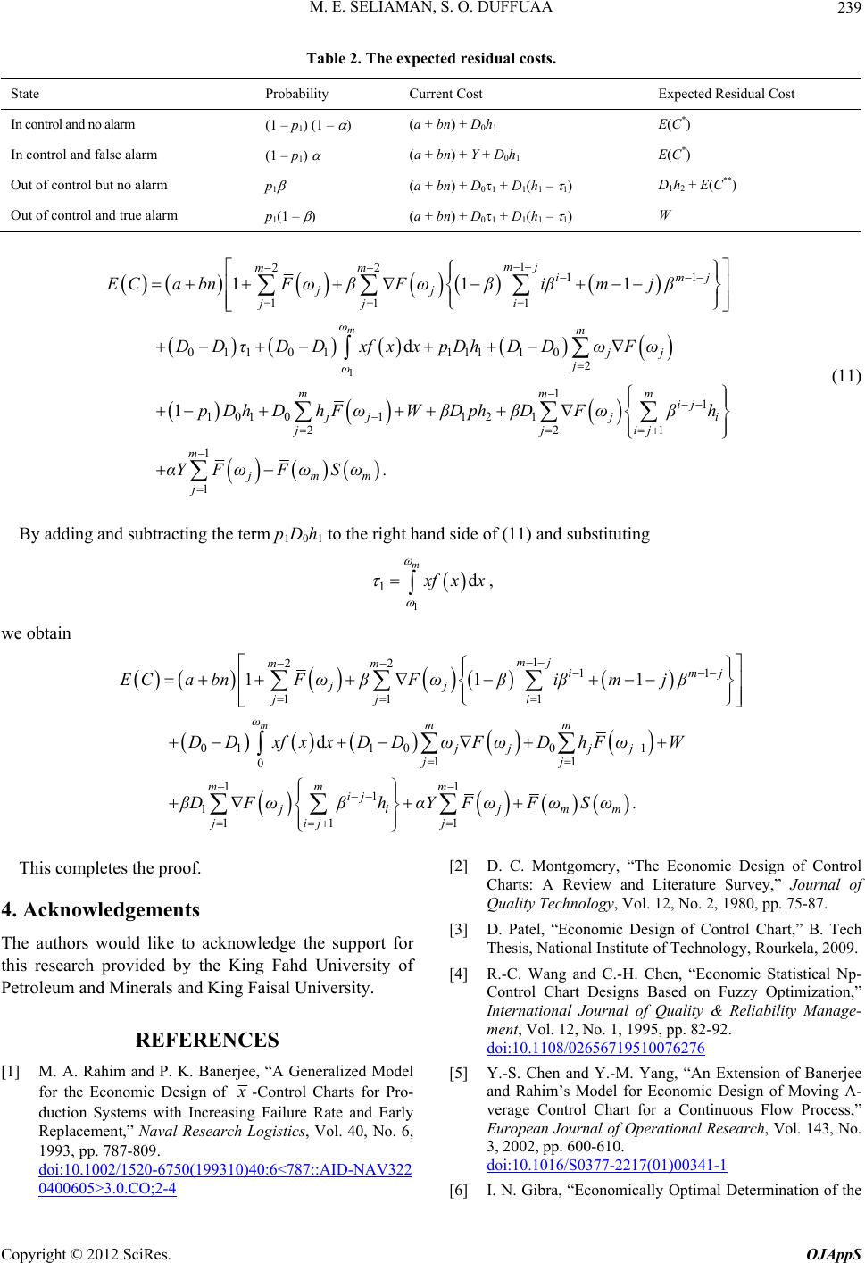

M. E. SELIAMAN, S. O. DUFFUAA 239

Table 2. The expected residual costs.

State Probability Expected Residual Cost Current Cost

In control and no alarm 1



) 1

(1 – p) (1 – (a + bn) + D0h E(C*)

In control and false alarm 0h1

h1 –



1) 2E(C**)



)

(1 – p1)



(a + bn) + Y + D E(C*)

Out of control but no alarm p1



(a + bn) + D01 + D1(D1h +

Out of control and true alarm p1(1 –(a + bn) + D01 + D1(h1 –



1) W

 

 

 





 

22 11

11 1

01101111 10

10101121

111

mm im

jj i

ωm

ECa bnFωβ Fωβiβmjβ

DDτDDxfxxpDh DDωFω

pDh DhFωWβDph βDFωβh



 

 













































 







 





















jmm

αYFωFωSω .













(11)

By adding and subtracting the term p1D0h1 to the right hand side of (11) and substituting



fx x





,



we obtain

 

 

 



 



22 11

11 1

011001

11 1

111

mm im

jj i

ωmm

jj jj

mm m

ji jmm

jijj

ECa bnFωβ Fωβiβmjβ

DD xfxxDDωFωDhFωW

βDFωβhαYFωFωSω .



 

 







 



j























 





 













 

This completes the proof.

4. Acknowledgements

cknowledge the support for

REFERENCES

[1] M. A. Rahim Generalized Mode

The authors would like to a

this research provided by the King Fahd University of

Petroleum and Minerals and King Faisal University.

and P. K. Banerjee, “A l

for the Economic Design of

-Control Charts for Pro-

duction Systems with Increasing Failure Rate and Early

Replacement,” Naval Research Logistics, Vol. 40, No. 6,

1993, pp. 787-809.

doi:10.1002/1520-6750(199310)40:6<787::AID-NAV322

0400605>3.0.CO;2-4

Charts: A Review an

[2] D. C. Montgomery, “The Economic Design of Control

d Literature Survey,” Journal of

09.

Quality Technology, Vol. 12, No. 2, 1980, pp. 75-87.

[3] D. Patel, “Economic Design of Control Chart,” B. Tech

Thesis, National Institute of Technology, Rourkela, 20

[4] R.-C. Wang and C.-H. Chen, “Economic Statistical Np-

Control Chart Designs Based on Fuzzy Optimization,”

International Journal of Quality & Reliability Manage-

ment, Vol. 12, No. 1, 1995, pp. 82-92.

doi:10.1108/02656719510076276

[5] Y.-S. Chen and Y.-M. Yang, “An Extension of Banerjee

and Rahim’s Model for Economic Design of Moving A-

verage Control Chart for a Continuous Flow Process,”

European Journal of Operational Research, Vol. 143, No.

3, 2002, pp. 600-610.

doi:10.1016/S0377-2217(01)00341-1

[6] I. N. Gibra, “Economically Optimal Determination of the

M. E. SELIAMAN, S. O. DUFFUAA

240

Parameters of

-Control Chart,” Management Sc

nd R Charts,” Tech-

ience,

Vol. 17, No. 9, 1971, pp. 635-646.

[7] E. M. Saniga, “Economic Statistical Control-Chart De-

signs with an Application to X a

nometrics, Vol. 31, No. 3, 1989, pp. 313-320.

[8] A. J. Duncan, “The Economic Design of

-Control

Charts Used to Maintain Current Control of a Process,”

Journal of the American Statistics Association, Vol. 51,

1956, pp. 228-242.

[9] P. K. Banerjee and M. A. Rahim, “Economic Design of

-Control Charts under Weibull Shock Models,” Tech-

nometrics, Vol. 30, No. 4, 1998, pp. 407-414.

Notation

Z0 = expected search time associated with a false alarm.

Z1 = expected search time to discover the assignable

cause and repair.

a = fixed sampling cost.

b = sampling cost per unit sampled.

Y = cost per false alarm.

W = cost to locate and repair the assignable cause.

D0 = quality cost per hour while producing and the pro-

cess is in control.

D1 = quality cost per hour while producing and the pro-

cess is out of control.



= probability of Type I error.



= probability of Type II error.

h = the sampling interval for a uniform sampling

scheme.

h = the jth sampling interval for a non-uniform sam-

pling scheme.



= h1 + h2 +···+ hj.

M = a specified number of sampling intervals.

n = sample size.

E(T) = expected cycle length.

E(C) = expected cost.

Pj = the conditional probability that process goes out of

control between 1





and



, given that it was at the

in-control state at time 1



