Weighted Time-Variant Slide Fuzzy Time-Series Models for Short-Term Load Forecasting

doi:10.4236/jilsa.2012.44030

Paper Menu >>

Journal Menu >>

Journal of Intelligent Learning Systems and Applications, 2012, 4, 285-290

http://dx.doi.org/10.4236/jilsa.2012.44030 Published Online November 2012 (http://www.SciRP.org/journal/jilsa)

285

Weighted Time-Variant Slide Fuzzy Time-Series Models

for Short-Term Load Forecasting

Xiaojuan Liu1,2, Enjian Bai1, Jian’an Fang1

1College of Information Science & Technology, Donghua University, Shanghai, China; 2Department of Mathematics and Physics,

Shanghai University of Electric Power, Shanghai, China.

Email: [email protected]

Received May 29th, 2012; revised June 26th, 2012; accepted July 3rd, 2012

ABSTRACT

Short-term load forecast plays an important role in the day-to-day operation and scheduling of generating units. Season

and temperature are the most important factors that affect the load change, but random factors such as big sport events

or popular TV shows can change demand consumption in particular hours, which will lead to sudden load changes. A

weighted time-variant slide fuzzy time-series model (WTVS) for short-term load forecasting is proposed to improve

forecasting accuracy. The WTVS model is divided into three parts, including the data preprocessing, the trend training

and the load forecasting. In the data preprocessing phase, the impact of random factors will be weakened by smoothing

the historical data. In the trend training and load forecasting phase, the seasonal factor and the weighted historical data

are introduced into the Time-variant Slide Fuzzy Time-series Models (TVS) for short-term load forecasting. The WTVS

model is tested on the load of the National Electric Power Company in Jordan. Results show that the proposed WTVS

model achieves a significant improvement in load forecasting accuracy as compared to TVS models.

Keywords: Load Forecasting; Fuzzy Time-Series; Weighted; Slide

1. Introduction

Load forecast has been a research topic for many decades

and the accuracy of load forecast is crucial to electricity

power industry due to its direct influence on generating

planning. Short-term load forecast means the forecast

time lead is in the range of hours to a few days ahead,

which plays an important role in the day-to-day operation

and scheduling of generating units. There are many fac-

tors that affect the load changes, such as calendar, wea-

ther, economical and random factors. For short-term load

forecast, weather and random factors are the most impor-

tant factors. Season and temperature are have the most

influence to the load due to the fact that changes in tem-

perature results in direct changes in energy consumption

by heating and cooling appliances. Random factors such

as big sport events or popular TV shows can change de-

mand consumption in particular hours, which will lead to

sudden load changes. A number of load forecasting mod-

els have been presented in the last decades. These models

can be divided into traditional approaches [1] and the ar-

tificial intelligence methods [2]. The former include re-

gression models, time series models et al, and the latter

provided many new tools for the forecasting of short-

term load such as neural networks [3-5], fuzzy logic [6,7],

support vector machines [8], expert systems [9], hybrid

method [10,11] et al. In recent years, many researchers

have used fuzzy time series models to handle load fore-

casting problems [12-15]. Liu et al. proposed a Time-

variant Slide Fuzzy Time-series Model (TVS) for short-

term load forecasting [13], the TVS model only uses his-

torical data to predict the load changes. Taking into ac-

count the affect of season, temperature, and random fac-

tors, a Weighted Time-variant Slide Fuzzy Time-series

Forecasting Model (WTVS) is presented. The WTVS

model is divided into three parts, including the data pre-

processing, the trend training and the load forecasting. In

the data preprocessing stage, the impact of random fac-

tors will be weakened by smoothing the history data. In

the trend training and load forecasting stage, the seasonal

factor and the weight of history data are introduced into

the TVS model. The WTVS model is tested on the load

of the National Electric Power Company in Jordan. Re-

sults show that the WTVS model achieves a significant

improvement in load forecasting accuracy as compared

to TVS models.

2. Time-Variant Fuzzy Time-Series

A fuzzy set

defined in the universe of discourse





12 ,

Uu u,,ucan be represented as











11AA2 2Ann

fuu fu ufu u,where A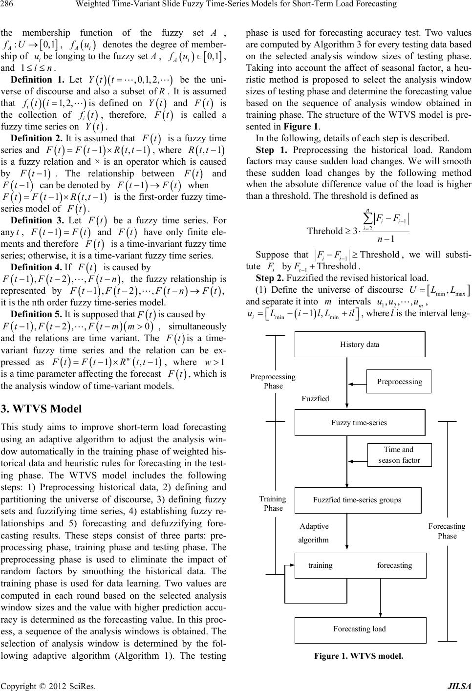

Weighted Time-Variant Slide Fuzzy Time-Series Models for Short-Term Load Forecasting

286

the membership function of the fuzzy set





:0,fU1



AiA,

u denotes the degree of member-

ship of be longing to the fuzzy set







0, 1

fu







and .

1in



1,fti

Definition 1. Let Yt be the uni-

verse of discourse and also a subset of. It is assumed

that iis defined on and



,0,t1,2,





2,





t is

the collection of



t, therefore,



t is called a

fuzzy time series on .





Definition 2. It is assumed that



t is a fuzzy time

series and

 





11Rtt,Ft Ft , where





Rt,1t



is a fuzzy relation and × is an operator which is caused

by . The relationship between



1Ft







and

can be denoted by



1Ft



tFt when

is the first-order fuzzy time-

series model of

 

Ft Ft

 

1



1,Rtt





Definition 3. Let



t be a fuzzy time series. For

any t,



tFt and



t have only finite ele-

ments and therefore



is a time-invariant fuzzy time

series; otherwise, it is a time-variant fuzzy time series.

Definition 4. If



2, ,

is caused by



 

tFtFtn







the fuzzy relationship is

represented by







1,2, ,,

tFtFtn tF



it is the nth order fuzzy time-series model.

Definition 5. It is supposed that

tis caused by

 





01,Ft Ft2, ,Ftmm, simultaneously

and the relations are time variant. The







is a time-

variant fuzzy time series and the relation can be ex-

pressed as , where

is a time parameter affecting the forecast

 

Ft



R





,tFt w



t, which is

the analysis window of time-variant models.

3. WTVS Model

This study aims to improve short-term load forecasting

using an adaptive algorithm to adjust the analysis win-

dow automatically in the training phase of weighted his-

torical data and heuristic rules for forecasting in the test-

ing phase. The WTVS model includes the following

steps: 1) Preprocessing historical data, 2) defining and

partitioning the universe of discourse, 3) defining fuzzy

sets and fuzzifying time series, 4) establishing fuzzy re-

lationships and 5) forecasting and defuzzifying fore-

casting results. These steps consist of three parts: pre-

processing phase, training phase and testing phase. The

preprocessing phase is used to eliminate the impact of

random factors by smoothing the historical data. The

training phase is used for data learning. Two values are

computed in each round based on the selected analysis

window sizes and the value with higher prediction accu-

racy is determined as the forecasting value. In this proc-

ess, a sequence of the analysis windows is obtained. The

selection of analysis window is determined by the fol-

lowing adaptive algorithm (Algorithm 1). The testing

phase is used for forecasting accuracy test. Two values

are computed by Algorithm 3 for every testing data based

on the selected analysis window sizes of testing phase.

Taking into account the affect of seasonal factor, a heu-

ristic method is proposed to select the analysis window

sizes of testing phase and determine the forecasting value

based on the sequence of analysis window obtained in

training phase. The structure of the WTVS model is pre-

sented in Figure 1.

In the following, details of each step is described.

Step 1. Preprocessing the historical load. Random

factors may cause sudden load changes. We will smooth

these sudden load changes by the following method

when the absolute difference value of the load is higher

than a threshold. The threshold is defined as

Threhold 31







 



Suppose that 1Threshold



 , we will substi-

tute t

by1Threshold

F



Step 2. Fuzzified the revised historical load.

(1) Define the universe of discourse





min max

,ULL

and separate it into intervals 12

uu , m,,





min n

uL iil



 







, wherelis the interval leng-

History data

Preprocessing

Fuzzfied

Fuzzy time-series

Fuzzfied time-series groups

Adaptive

algorithm

Forecasting load

training forecasting

Time and

season factor

Preprocessing

Phase

Training

Phase

Forecasting

Phase

Figure 1. WTVS model.

Weighted Time-Variant Slide Fuzzy Time-Series Models for Short-Term Load Forecasting 287

th, the midpoint ofis .

i i

(2) Define the fuzzy sets

u m

and fuzzify the data.

 



1, 2,,

ii i

AA Am

fu fufu

uu u

 

Step 3. Establishing fuzzy relationships of time

and and group the fuzzy time-series.

1t

In the training phase, the fuzzy relationship is sup-

posed to be ij

A. In the testing phase, the fuzzy

relationship is supposed to be .

A

Generally, the trend of load in summer and winter is

shown in Tables 1 and 2, respectively. For example, in

summer, we can conclude that from 1 to 6 o’clock, the

load have the downward trend, while from 7 to 12

o’clock, the load have the upward trend. These trends can

be used to revise the forecast in the forecasting phase.

Step 4. Forecasting and defuzzifying forecasting re-

sults.

In the training phase, each round calculates values For

1 and For 2 and compares the two values to actual value

Act with the better one as the forecasting load. The ana-

lysis window is determined by Algorithm 1. The compu-

tations of For 1 and For 2 are carried out by Algorithm 2.

In the testing phase, the forecasting load is determined by

Algorithm 3.

Algorithm 1. (slide analysis window)

(1) ;; 1, whereand1i1

S2

Si

S1i



are the

sizes of the initial window. Flag .

1n

(2) If the prediction accuracy computed by 1i



higher than that of i, then slide the analysis window

forward and the size of the analysis window plus 1, and

flag . Otherwise, slide the analysis window

backward and the size of the analysis window minus 1,

and flag .

1nn

nn1

(3) Repeat step (2) until the end of the training data.

Algorithm 2. (training phase) Suppose that the fuzzy

relationship of time and is j

k1ki

A, and the

analysis window size is . Let





be the middle

value of interval

(1) Select two initial window sizes 11S



and

. Let .

22S1n

1For

(2) If,

n1





. If , 2n

Table 1. Load trend in summer.

Time 1 - 6 7 - 12 13 - 20 21 - 24

Trend ↓ ↑ ↓ ↓

Table 2. Load trend in winter.

Time 1 - 6 7 - 12 13 - 16 17 - 18 19 - 24

Trend ↓ ↑ ↓ ↑ ↓



For 2

ttiti

iFFM

nnn







 



 A





 





















 ,

where 1111

,,, ,1,2,3,4

8642







 







and





t is the actual load at time . t



tti

DFiFFu

nnn











tij















then





, and 1



. Else



, and



(3) Compared with the actual load, if the training ac-

curacy of theis higher than, then

For 2

For 1

predict ForF



. Else .

predict

(4) Slide the analysis window until the end of the

whole training data.

ForF1

Algorithm 3. (forecasting phase ) Suppose that the

fuzzy relationship of timekand is, and the

analysis window size is n. let

1k#

A







1

be the middle

value of intervalu.

(1) Select two initial window sizes and

S22S



Let 1n



(2) If 1n







For 3i

A. If, 2n



For 4

FiFF

nnn







 iti







 























where 11 11

,,, ,1,2,3,4

8642















and





tis the actual load at time. t



tti

DFiFFu

nnn











tij















Then





, and 1



. Else



, and



(3) Consider the trend of load change and the sequence

of flags which obtained in training phase, there are the

following heuristic rules:

1) If 1tt



, and the actual load at timetis bigger

than that of time 1t



, then the load at time 1t



has

the trend of increasing. At the same time pay attention to

the trend in Tables 1 and 2, the forecast value is max





For 4

For 3.

2) If 1tt





,and the actual load at time is smaller

than that of time



, then the load at time 1t



has

the trend of decreasing. At the same time pay attention to

the trend in Tables 1 and 2, the forecast value is min





For4For 3.

3) Else, the forecast value is the arithmetic average of

For 3 and For 4.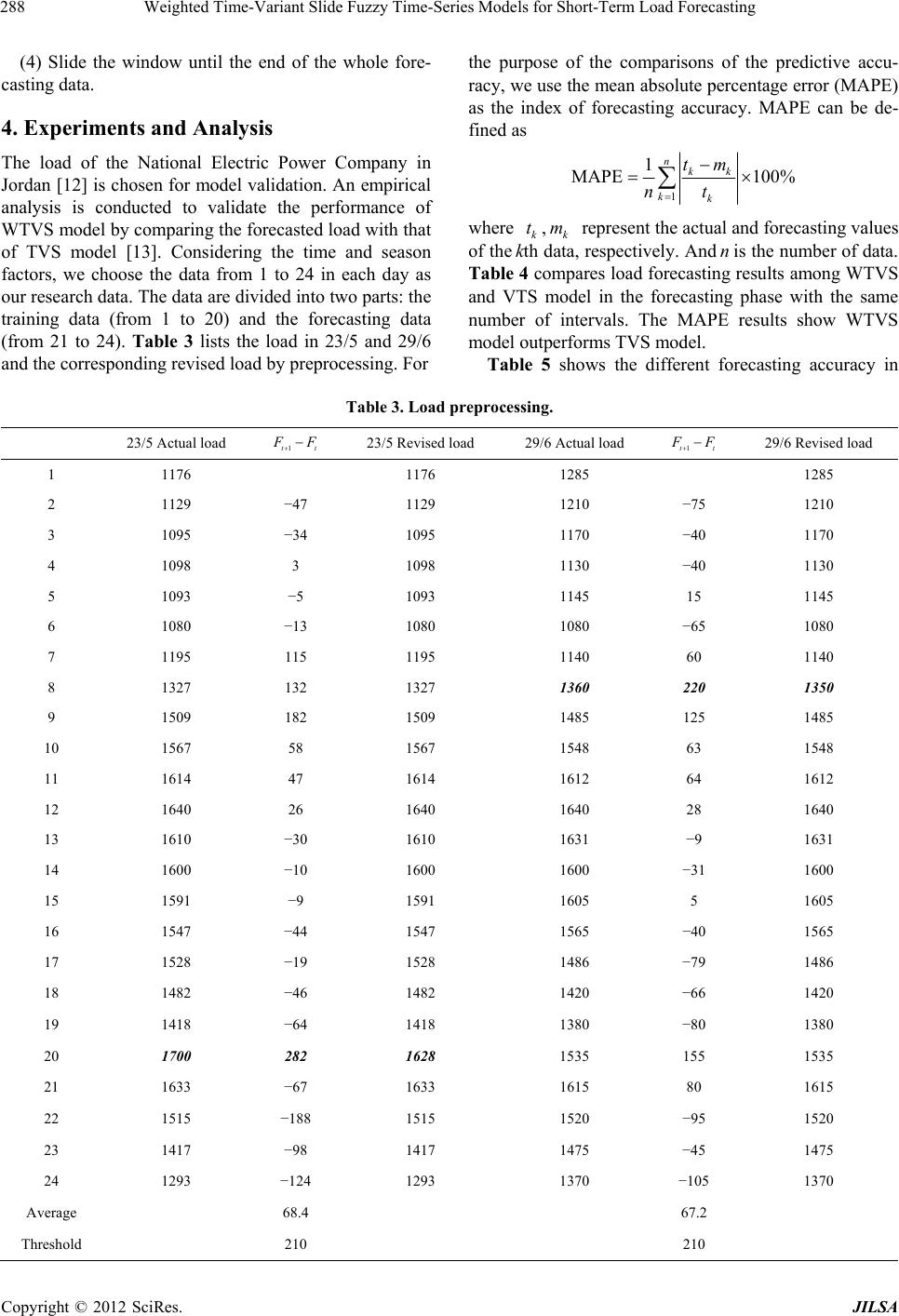

Weighted Time-Variant Slide Fuzzy Time-Series Models for Short-Term Load Forecasting

288

(4) Slide the window until the end of the whole fore-

casting data.

the purpose of the comparisons of the predictive accu-

racy, we use the mean absolute percentage error (MAPE)

as the index of forecasting accuracy. MAPE can be de-

fined as

4. Experiments and Analysis

The load of the National Electric Power Company in

Jordan [12] is chosen for model validation. An empirical

analysis is conducted to validate the performance of

WTVS model by comparing the forecasted load with that

of TVS model [13]. Considering the time and season

factors, we choose the data from 1 to 24 in each day as

our research data. The data are divided into two parts: the

training data (from 1 to 20) and the forecasting data

(from 21 to 24). Table 3 lists the load in 23/5 and 29/6

and the corresponding revised load by preprocessing. For

MAPE 100%

nkk









where ,k represent the actual and forecasting values

of thedata, respectively. Andnis the number of data.

Table 4 compares load forecasting results among WTVS

and VTS model in the forecasting phase with the same

number of intervals. The MAPE results show WTVS

model outperforms TVS model.

thkm

Table 5 shows the different forecasting accuracy in

Table 3. Load preprocessing.

23/5 Actual load 1tt

 23/5 Revised load 29/6 Actual load 1tt

 29/6 Revised load

1 1176 1176 1285 1285

2 1129 −47 1129 1210 −75 1210

3 1095 −34 1095 1170 −40 1170

4 1098 3 1098 1130 −40 1130

5 1093 −5 1093 1145 15 1145

6 1080 −13 1080 1080 −65 1080

7 1195 115 1195 1140 60 1140

8 1327 132 1327 1360 220 1350

9 1509 182 1509 1485 125 1485

10 1567 58 1567 1548 63 1548

11 1614 47 1614 1612 64 1612

12 1640 26 1640 1640 28 1640

13 1610 −30 1610 1631 −9 1631

14 1600 −10 1600 1600 −31 1600

15 1591 −9 1591 1605 5 1605

16 1547 −44 1547 1565 −40 1565

17 1528 −19 1528 1486 −79 1486

18 1482 −46 1482 1420 −66 1420

19 1418 −64 1418 1380 −80 1380

20 1700 282 1628 1535 155 1535

21 1633 −67 1633 1615 80 1615

22 1515 −188 1515 1520 −95 1520

23 1417 −98 1417 1475 −45 1475

24 1293 −124 1293 1370 −105 1370

Average 68.4 67.2

Threshold 210 210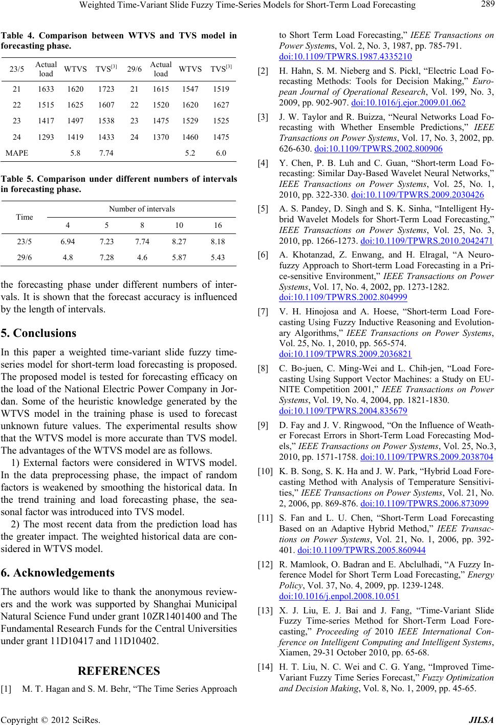

Weighted Time-Variant Slide Fuzzy Time-Series Models for Short-Term Load Forecasting 289

Table 4. Comparison between WTVS and TVS model in

forecasting phase.

23/5 Actual

load WTVS TVS[3] 29/6

Actual

load WTVS TVS[3]

21 1633 1620 1723 21 1615 15471519

22 1515 1625 1607 22 1520 16201627

23 1417 1497 1538 23 1475 15291525

24 1293 1419 1433 24 1370 14601475

MAPE 5.8 7.74 5.2 6.0

Table 5. Comparison under different numbers of intervals

in forecasting phase.

Number of intervals

Time

4 5 8 10 16

23/5 6.94 7.23 7.74 8.27 8.18

29/6 4.8 7.28 4.6 5.87 5.43

the forecasting phase under different numbers of inter-

vals. It is shown that the forecast accuracy is influenced

by the length of intervals.

5. Conclusions

In this paper a weighted time-variant slide fuzzy time-

series model for short-term load forecasting is proposed.

The proposed model is tested for forecasting efficacy on

the load of the National Electric Power Company in Jor-

dan. Some of the heuristic knowledge generated by the

WTVS model in the training phase is used to forecast

unknown future values. The experimental results show

that the WTVS model is more accurate than TVS model.

The advantages of the WTVS model are as follows.

1) External factors were considered in WTVS model.

In the data preprocessing phase, the impact of random

factors is weakened by smoothing the historical data. In

the trend training and load forecasting phase, the sea-

sonal factor was introduced into TVS model.

2) The most recent data from the prediction load has

the greater impact. The weighted historical data are con-

sidered in WTVS model.

6. Acknowledgements

The authors would like to thank the anonymous review-

ers and the work was supported by Shanghai Municipal

Natural Science Fund under grant 10ZR1401400 and The

Fundamental Research Funds for the Central Universities

under grant 11D10417 and 11D10402.

REFERENCES

[1] M. T. Hagan and S. M. Behr, “The Time Series Approach

to Short Term Load Forecasting,” IEEE Transactions on

Power Systems, Vol. 2, No. 3, 1987, pp. 785-791.

doi:10.1109/TPWRS.1987.4335210

[2] H. Hahn, S. M. Nieberg and S. Pickl, “Electric Load Fo-

recasting Methods: Tools for Decision Making,” Euro-

pean Journal of Operational Research, Vol. 199, No. 3,

2009, pp. 902-907. doi:10.1016/j.ejor.2009.01.062

[3] J. W. Taylor and R. Buizza, “Neural Networks Load Fo-

recasting with Whether Ensemble Predictions,” IEEE

Transactions on Power Systems, Vol. 17, No. 3, 2002, pp.

626-630. doi:10.1109/TPWRS.2002.800906

[4] Y. Chen, P. B. Luh and C. Guan, “Short-term Load Fo-

recasting: Similar Day-Based Wavelet Neural Networks,”

IEEE Transactions on Power Systems, Vol. 25, No. 1,

2010, pp. 322-330. doi:10.1109/TPWRS.2009.2030426

[5] A. S. Pandey, D. Singh and S. K. Sinha, “Intelligent Hy-

brid Wavelet Models for Short-Term Load Forecasting,”

IEEE Transactions on Power Systems, Vol. 25, No. 3,

2010, pp. 1266-1273. doi:10.1109/TPWRS.2010.2042471

[6] A. Khotanzad, Z. Enwang, and H. Elragal, “A Neuro-

fuzzy Approach to Short-term Load Forecasting in a Pri-

ce-sensitive Environment,” IEEE Transactions on Power

Systems, Vol. 17, No. 4, 2002, pp. 1273-1282.

doi:10.1109/TPWRS.2002.804999

[7] V. H. Hinojosa and A. Hoese, “Short-term Load Fore-

casting Using Fuzzy Inductive Reasoning and Evolution-

ary Algorithms,” IEEE Transactions on Power Systems,

Vol. 25, No. 1, 2010, pp. 565-574.

doi:10.1109/TPWRS.2009.2036821

[8] C. Bo-juen, C. Ming-Wei and L. Chih-jen, “Load Fore-

casting Using Support Vector Machines: a Study on EU-

NITE Competition 2001,” IEEE Transactions on Power

Systems, Vol. 19, No. 4, 2004, pp. 1821-1830.

doi:10.1109/TPWRS.2004.835679

[9] D. Fay and J. V. Ringwood, “On the Influence of Weath-

er Forecast Errors in Short-Term Load Forecasting Mod-

els,” IEEE Transactions on Power Systems, Vol. 25, No.3,

2010, pp. 1571-1758. doi:10.1109/TPWRS.2009.2038704

[10] K. B. Song, S. K. Ha and J. W. Park, “Hybrid Load Fore-

casting Method with Analysis of Temperature Sensitivi-

ties,” IEEE Transactions on Power Systems, Vol. 21, No.

2, 2006, pp. 869-876. doi:10.1109/TPWRS.2006.873099

[11] S. Fan and L. U. Chen, “Short-Term Load Forecasting

Based on an Adaptive Hybrid Method,” IEEE Transac-

tions on Power Systems, Vol. 21, No. 1, 2006, pp. 392-

401. doi:10.1109/TPWRS.2005.860944

[12] R. Mamlook, O. Badran and E. Abclulhadi, “A Fuzzy In-

ference Model for Short Term Load Forecasting,” Energy

Policy, Vol. 37, No. 4, 2009, pp. 1239-1248.

doi:10.1016/j.enpol.2008.10.051

[13] X. J. Liu, E. J. Bai and J. Fang, “Time-Variant Slide

Fuzzy Time-series Method for Short-Term Load Fore-

casting,” Proceeding of 2010 IEEE International Con-

ference on Intelligent Computing and Intelligent Systems,

Xiamen, 29-31 October 2010, pp. 65-68.

[14] H. T. Liu, N. C. Wei and C. G. Yang, “Improved Time-

Variant Fuzzy Time Series Forecast,” Fuzzy Optimization

and Decision Making, Vol. 8, No. 1, 2009, pp. 45-65.

Weighted Time-Variant Slide Fuzzy Time-Series Models for Short-Term Load Forecasting

290

doi:10.1007/s10700-009-9051-8

[15] C. A. Maia and M. Goncalves, “Application of Switched

Adaptive System to Load Forecasting,” Electric Power

Systems Research, Vol. 78, No. 4, 2008, pp. 721-727.

doi:10.1016/j.epsr.2007.05.014