Comparison between Neural Network and Adaptive Neuro-Fuzzy Inference System for Forecasting Chaotic Traffic Volumes

doi:10.4236/jilsa.2012.44025

Paper Menu >>

Journal Menu >>

Journal of Intelligent Learning Systems and Applications, 2012, 4, 247-254

http://dx.doi.org/10.4236/jilsa.2012.44025 Published Online November 2012 (http://www.SciRP.org/journal/jilsa)

247

Comparison between Neural Network and Adaptive

Neuro-Fuzzy Inference System for Forecasting Chaotic

Traffic Volumes

Jiin-Po Yeh1, Yu-Chen Chang2

1Department of Civil and Ecological Engineering, I-Shou University, Kaohsiung City, Taiwan; 2Institute of Civil Engineering Tech-

nology, National Kaohsiung University of Applied Sciences, Kaohsiung City, Taiwan.

Email: [email protected]

Received May 26th, 2012; revised June 19th, 2012; accepted June 26th, 2012

ABSTRACT

This paper applies both the neural network and adaptive neuro-fuzzy inference system for forecasting short-term chaotic

traffic volumes and compares the results. The architecture of the neural network consists of the input vector, one hidden

layer and output layer. Bayesian regularization is employed to obtain the effective number of neurons in the hidden

layer. The input variables and target of the adaptive neuro-fuzzy inference system are the same as those of the neural

network. The data clustering technique is used to group data points so that the membership functions will be more tai-

lored to the input data, which in turn greatly reduces the number of fuzzy rules. Numerical results indicate that these

two models have almost the same accuracy, while the adaptive neuro-fuzzy inference system takes more time to train. It

is also shown that although the effective number of neurons in the hidden layer is less than half the number of the input

elements, the neural network can have satisfactory performance.

Keywords: Neural Network; Adaptive Neuro-Fuzzy Inference System; Chaotic Traffic Volumes; State Space

Reconstruction

1. Introduction

It has been known for decades that chaotic behaviors

exist in traffic flow systems Gazis et al. [1] developed a

generalized car-following model, known as the GHR (Ga-

zis-Herman-Rothery) model, whose discontinuous beha-

vior and nonlinearity suggested chaotic solutions for a

certain range of input parameters. Due to the capacity di-

mension [2] of the attractor being fractal and first Lyapu-

nov exponent [3] being positive, Disbro and Frame [4]

showed the presence of chaos in this General Motors’ mo-

del without signals, bottlenecks, intersections, etc. or with

a coordinated signal network. Chaos was observed in a

platoon of vehicles described by the traditional GHR mo-

del modified by adding a nonlinear inter-car separation

dependent term [5,6], Poincaré maps of which appear as a

cloud of points without any repeat. Traffic volume col-

lected at 2-min interval on the Beijing Xizhimen highway,

China, was also found to posses chaotic behaviors [7].

Because of nonperiodic behaviors, chaotic time series

seem to be unpredictable, but a variety of short-term

forecast models have been attempted and proven to be

successful, such as models employing Kalman filtering

theory [8], the local linear model using information based

on past values [9], the polynomial model [10], neural

network-based black-box models [11-15], a model con-

sisting of a fuzzy C-means clustering and a radial-ba-

sis-function neural network [16], etc. This paper also

tries to forecast the short-term chaotic traffic volume at

the intersection. Two kinds of models are presented for

comparison. One is the neural network, where the delay

coordinates [2,17,18] of the reconstructed state space of

the traffic flow system are used as the input vector of the

neural network and the first delay coordinate of next state

as the target of the neural network. The other model is

the adaptive neuro-fuzzy inference system [19,20], where

inputs and targets are identical to the first one, but mem-

bership functions and fuzzy rules [21,22] replace neurons

in the neural network. The number and the shapes of the

membership functions are decided and tuned by a data

clustering technique and backpropagation neural network,

respectively, which is different from the Park’s model

[16] in the ways of data clustering and learning process.

2. Diagnosis of Chaos

The Poincaré map, time series, autocorrelation function,

etc., can often provide graphic evidence for chaotic be-

Comparison between Neural Network and Adaptive Neuro-Fuzzy Inference System for

Forecasting Chaotic Traffic Volumes

248

havior, while the fractal dimension and largest Lyapunov

exponent are two principal quantitative measures of chaos.

This paper selects the fractal dimension, largest Lyapu-

nov exponent and autocorrelation function to show the

existence of chaos of the traffic flow. Brief introduction

to them is as follows.

2.1. Fractal Dimension

If there is only one measurement available for a system,

delay coordinates are usually used to reconstruct its state

space [17]. Given a time series x(t) and time delay



, an

n-dimensional state space can be reconstructed with the

delay coordinates:

  





{,,2,, 1xt xtxtxtn









 . To get

the appropriate dimension for reconstructing the state

space of a chaotic dynamical system, the first step is to

obtain the fractal dimension of the chaotic attractor in the

state space. There are a number of ways to measure the

chaotic attractor dimension [2]. Among them, this paper

chose the method of correlation dimension, because it is

much easier to implement and not time-consuming. Con-

sider an orbit discretized to a set of N points in the state

space. A sphere of radius r is poisoned at each point of

the orbit and the number of points within each sphere

with Euclidean distance less than r is counted. A correla-

tion function is then defined as [2,23]

 



lim

1ij

nij

CrHri j





 XX (1)

where ij

is the Euclidean distance between

points Xi and Xj and H is the Heaviside function (or unit

step function ). For many attractors, this function C(r)

exhibits a power law dependence on r, as ; that is

XX

0r



lim d

rCr ar

 (2)

Hence, a correlation dimension is defined by the expres-

sion



lim ln



 (3)

The chaotic attractor dimension will often approach an

asymptote d with the dimension of the reconstructed state

space gradually increasing. To embed a d-dimensional

chaotic attractor, the state space may be reconstructed

with dimension greater than or equal to 2d + 1, which ac-

cording to Takens [24] will be sufficient to have generic

delay plots.

2.2. The Largest Lyapunov Exponent

The largest Lyapunov exponent of a chaotic orbit is de-

fined by the expression [3]

lim log

mii



 

 (4)

The calculation is initiated by locating the nearest

neighbor to the first point of a reference trajectory in the

reconstructed state space and the distance between them

is denoted by d0i. This pair of points is then propagated

through the attractor for a fixed short time  and its final

separation di is computed. After that, a replacement for

the propagated pair is attempted by the following proce-

dure: 1) The distance of each delay coordinate point in

the attractor to the propagated point of the reference tra-

jectory is determined; 2) Points closer than a given length

and away from another much smaller length (to avoid

noise) are examined to see if the angle between the

original pair and attempted pairs is less than a given

small angle (e.g. 0.3 radians); and 3) The attempted pair

with the smallest angle is used as replacement for the

next propagation. The repeating of propagating and re-

placing are carried out for m cycles.

2.3. Autocorrelation Function

To find out the resemblance of the signal





t with

itself as time passes, the autocorrelation function

 

lim d

Rxtxt







t





(5)

is an often-seen tool to achieve this purpose. If







approaches the square of the mean of the function







, it means that the signal is only correlated

with its recent past [25], i.e., sensitive to the initial con-

ditions. Furthermore, the time lag



at which







first crosses the square of the mean of the function





is usually considered as the time delay



for recon-

structing the state space.

3. Forecasting Models

There are two models applied in this paper to forecast

short-term chaotic traffic volumes: the feedforward back-

propgation neural network and the adaptive neuro-fuzzy

inference system, which are described as follows.

3.1. Feedforward Backpropagation Neural

Network Model

The first forecasting model used in this paper is a feed-

forward neural network with the backpropagation train-

ing algorithm, as shown in Figure 1. The transfer func-

tion in the single hidden layer is the tan-sigmoid function



1e ,1,2,3,,

ii n

afni s



 

 (6)

where ,1 1,22,12R

,,,,

ii iiRRi

nwxwxwxbxxx



 

are the elements of the input vector, s is the number of

Co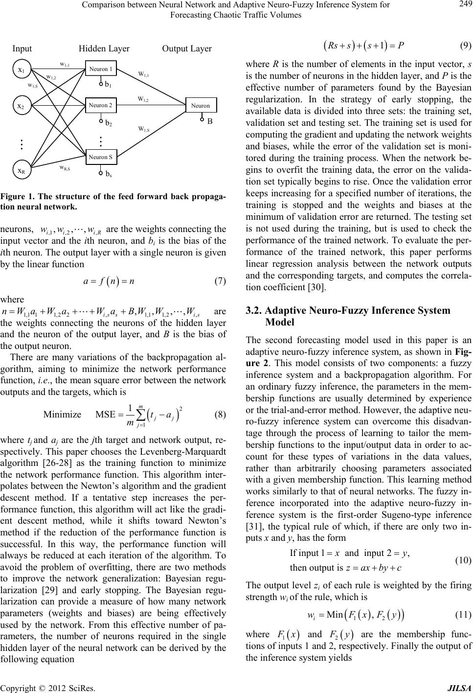mparison between Neural Network and Adaptive Neuro-Fuzzy Inference System for

Forecasting Chaotic Traffic Volumes

249

Neuron 1

Neuron 2

Neuron S

w1,1

Neuron

w1,2

w1,S

wR,S

W1,1

W1,2

W1,S

Input Hidden Layer Output Layer

Figure 1. The structure of the feed forward back propaga-

tion neural network.

neurons, ,1, 2, R

are the weights connecting the

input vector and the ith neuron, and bi is the bias of the

ith neuron. The output layer with a single neuron is given

by the linear function

,,,

ii i

ww w



afn n (7)

where

1,1 11,22,1,11,2, are

the weights connecting the neurons of the hidden layer

and the neuron of the output layer, and B is the bias of

the output neuron.

,, ,,

is sis

nWaWaWa BWWW 

There are many variations of the backpropagation al-

gorithm, aiming to minimize the network performance

function, i.e., the mean square error between the network

outputs and the targets, which is



Minimize MSE

m







(8)

where tj and aj are the jth target and network output, re-

spectively. This paper chooses the Levenberg-Marquardt

algorithm [26-28] as the training function to minimize

the network performance function. This algorithm inter-

polates between the Newton’s algorithm and the gradient

descent method. If a tentative step increases the per-

formance function, this algorithm will act like the gradi-

ent descent method, while it shifts toward Newton’s

method if the reduction of the performance function is

successful. In this way, the performance function will

always be reduced at each iteration of the algorithm. To

avoid the problem of overfitting, there are two methods

to improve the network generalization: Bayesian regu-

larization [29] and early stopping. The Bayesian regu-

larization can provide a measure of how many network

parameters (weights and biases) are being effectively

used by the network. From this effective number of pa-

rameters, the number of neurons required in the single

hidden layer of the neural network can be derived by the

following equation



 

1Rs ssP



 (9)

where R is the number of elements in the input vector, s

is the number of neurons in the hidden layer, and P is the

effective number of parameters found by the Bayesian

regularization. In the strategy of early stopping, the

available data is divided into three sets: the training set,

validation set and testing set. The training set is used for

computing the gradient and updating the network weights

and biases, while the error of the validation set is moni-

tored during the training process. When the network be-

gins to overfit the training data, the error on the valida-

tion set typically begins to rise. Once the validation error

keeps increasing for a specified number of iterations, the

training is stopped and the weights and biases at the

minimum of validation error are returned. The testing set

is not used during the training, but is used to check the

performance of the trained network. To evaluate the per-

formance of the trained network, this paper performs

linear regression analysis between the network outputs

and the corresponding targets, and computes the correla-

tion coefficient [30].

3.2. Adaptive Neuro-Fuzzy Inference System

Model

The second forecasting model used in this paper is an

adaptive neuro-fuzzy inference system, as shown in Fig-

ure 2. This model consists of two components: a fuzzy

inference system and a backpropagation algorithm. For

an ordinary fuzzy inference, the parameters in the mem-

bership functions are usually determined by experience

or the trial-and-error method. However, the adaptive neu-

ro-fuzzy inference system can overcome this disadvan-

tage through the process of learning to tailor the mem-

bership functions to the input/output data in order to ac-

count for these types of variations in the data values,

rather than arbitrarily choosing parameters associated

with a given membership function. This learning method

works similarly to that of neural networks. The fuzzy in-

ference incorporated into the adaptive neuro-fuzzy in-

ference system is the first-order Sugeno-type inference

[31], the typical rule of which, if there are only two in-

puts x and y, has the form

If input1and input 2,

then output is

zaxbyc



 (10)

The output level zi of each rule is weighted by the firing

strength wi of the rule, which is

 





Min ,

wFxFy

(11)

where





x and





y are the membership func-

tions of inputs 1 and 2, respectively. Finally the output of

the inference system yields

Co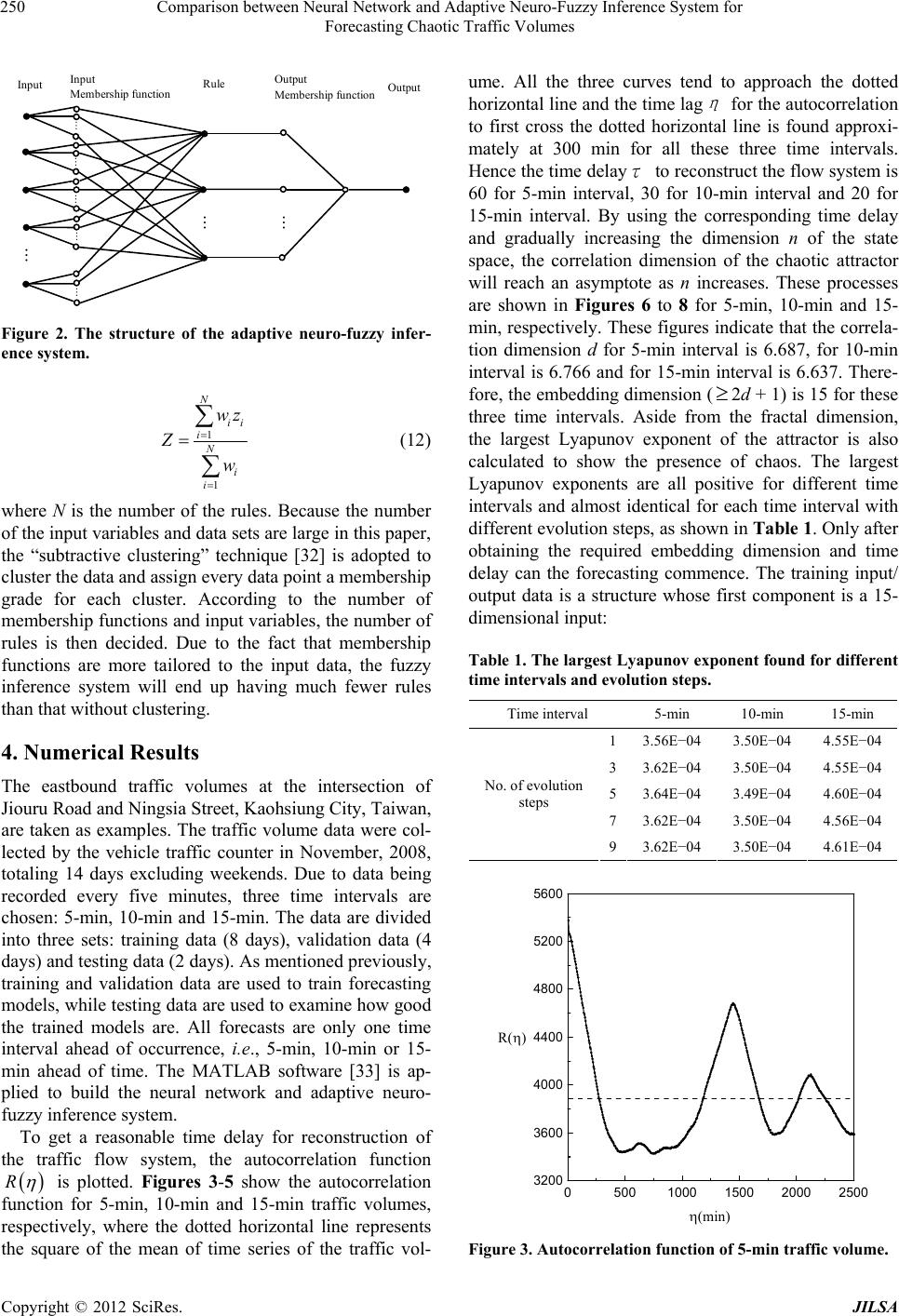mparison between Neural Network and Adaptive Neuro-Fuzzy Inference System for

Forecasting Chaotic Traffic Volumes

250

Input Input

Membership function Rule Output

Membership function Output

Figure 2. The structure of the adaptive neuro-fuzzy infer-

ence system.







(12)

where N is the number of the rules. Because the number

of the input variables and data sets are large in this paper,

the “subtractive clustering” technique [32] is adopted to

cluster the data and assign every data point a membership

grade for each cluster. According to the number of

membership functions and input variables, the number of

rules is then decided. Due to the fact that membership

functions are more tailored to the input data, the fuzzy

inference system will end up having much fewer rules

than that without clustering.

4. Numerical Results

The eastbound traffic volumes at the intersection of

Jiouru Road and Ningsia Street, Kaohsiung City, Taiwan,

are taken as examples. The traffic volume data were col-

lected by the vehicle traffic counter in November, 2008,

totaling 14 days excluding weekends. Due to data being

recorded every five minutes, three time intervals are

chosen: 5-min, 10-min and 15-min. The data are divided

into three sets: training data (8 days), validation data (4

days) and testing data (2 days). As mentioned previously,

training and validation data are used to train forecasting

models, while testing data are used to examine how good

the trained models are. All forecasts are only one time

interval ahead of occurrence, i.e., 5-min, 10-min or 15-

min ahead of time. The MATLAB software [33] is ap-

plied to build the neural network and adaptive neuro-

fuzzy inference system.

To get a reasonable time delay for reconstruction of

the traffic flow system, the autocorrelation function





is plotted. Figures 3-5 show the autocorrelation

function for 5-min, 10-min and 15-min traffic volumes,

respectively, where the dotted horizontal line represents

the square of the mean of time series of the traffic vol-

ume. All the three curves tend to approach the dotted

horizontal line and the time lag

for the autocorrelation

to first cross the dotted horizontal line is found approxi-

mately at 300 min for all these three time intervals.

Hence the time delayτ to reconstruct the flow system is

60 for 5-min interval, 30 for 10-min interval and 20 for

15-min interval. By using the corresponding time delay

and gradually increasing the dimension n of the state

space, the correlation dimension of the chaotic attractor

will reach an asymptote as n increases. These processes

are shown in Figures 6 to 8 for 5-min, 10-min and 15-

min, respectively. These figures indicate that the correla-

tion dimension d for 5-min interval is 6.687, for 10-min

interval is 6.766 and for 15-min interval is 6.637. There-

fore, the embedding dimension (2d + 1) is 15 for these

three time intervals. Aside from the fractal dimension,

the largest Lyapunov exponent of the attractor is also

calculated to show the presence of chaos. The largest

Lyapunov exponents are all positive for different time

intervals and almost identical for each time interval with

different evolution steps, as shown in Table 1. Only after

obtaining the required embedding dimension and time

delay can the forecasting commence. The training input/

output data is a structure whose first component is a 15-

dimensional input:

Table 1. The largest Lyapunov e xponent found for different

time intervals and evolution steps.

Time interval 5-min 10-min 15-min

1 3.56E−04 3.50E−04 4.55E−04

3 3.62E−04 3.50E−04 4.55E−04

5 3.64E−04 3.49E−04 4.60E−04

7 3.62E−04 3.50E−04 4.56E−04

No. of evolution

steps

9 3.62E−04 3.50E−04 4.61E−04

05001000 1500 20002500

3200

3600

4000

4400

4800

5200

5600



(min)

(



)

Figure 3. Autocorrelation function of 5-min traffic volume.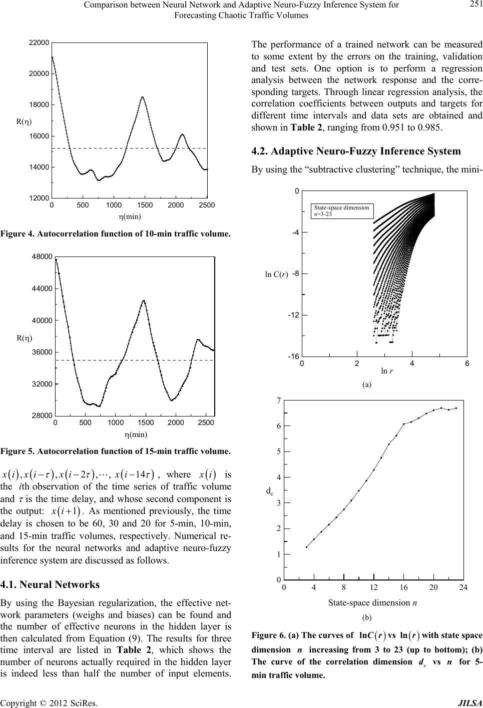

Comparison between Neural Network and Adaptive Neuro-Fuzzy Inference System for

Forecasting Chaotic Traffic Volumes

251

05001000 1500 2000 2500

12000

14000

16000

18000

20000

22000

(



)



(

in)

Figure 4. Autocorrelation function of 10-min traffic volume.

05001000 1500 20002500

2 8000

3 2000

3 6000

4 0000

4 4000

4 8000



(

)



)

Figure 5. Autocorrelation function of 15-min traffic volume.

















,,2,, 1xi xixixi4





 , where





i is

the observation of the time series of traffic volume

and



is the time delay, and whose second component is

the output:

thi





1xi. As mentioned previously, the time

delay is chosen to be 60, 30 and 20 for 5-min, 10-min,

and 15-min traffic volumes, respectively. Numerical re-

sults for the neural networks and adaptive neuro-fuzzy

inference system are discussed as follows.

4.1. Neural Networks

By using the Bayesian regularization, the effective net-

work parameters (weighs and biases) can be found and

the number of effective neurons in the hidden layer is

then calculated from Equation (9). The results for three

time interval are listed in Table 2, which shows the

number of neurons actually required in the hidden layer

is indeed less than half the number of input elements.

The performance of a trained network can be measured

to some extent by the errors on the training, validation

and test sets. One option is to perform a regression

analysis between the network response and the corre-

sponding targets. Through linear regression analysis, the

correlation coefficients between outputs and targets for

different time intervals and data sets are obtained and

shown in Table 2, ranging from 0.951 to 0.985.

4.2. Adaptive Neuro-Fuzzy Inference System

By using the “subtractive clustering” technique, the mini-

0246

-16

-12

-8

-4

ln C(

)

State-space dimension

=3-23

(a)

048 12162024

State-s

ace dimension

(b)

Figure 6. (a) The curves of





lnCrvs with state space

dimension increasing from 3 to 23 (up to bottom); (b)

The curve of the correlation dimension vs for 5-

min traffic volume.



ln r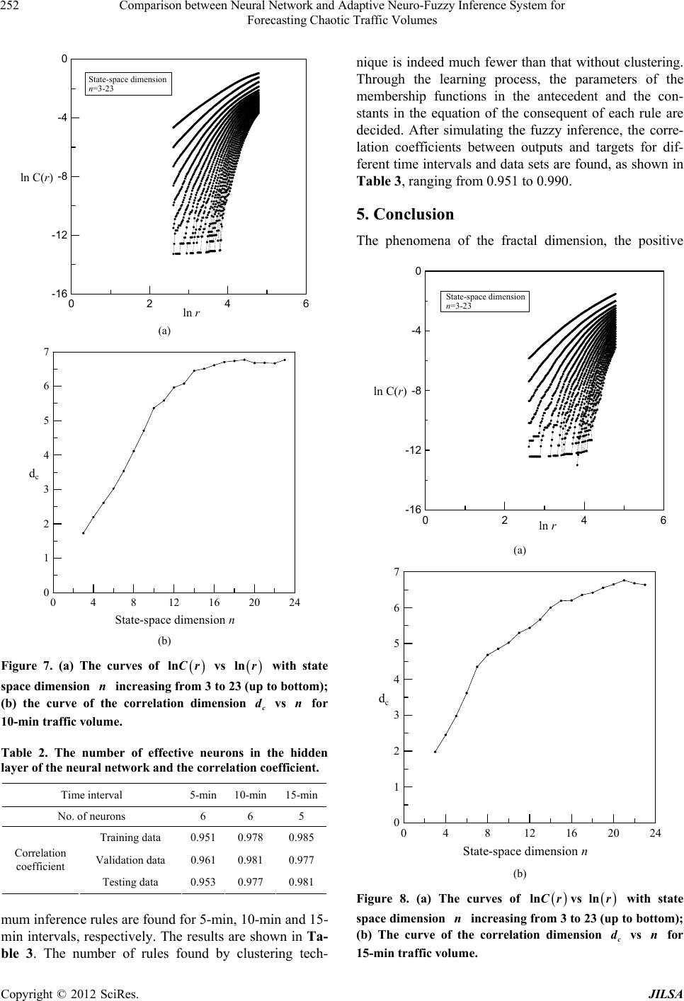

Comparison between Neural Network and Adaptive Neuro-Fuzzy Inference System for

Forecasting Chaotic Traffic Volumes

252

0246

-16

-12

-8

-4

ln C(

)

State-space dimension

=3-23

(a)

04812 16 20 24

State-s

ace dimension

(b)

Figure 7. (a) The curves of vs with state

space dimension increasing from 3 to 23 (up to bottom);

(b) the curve of the correlation dimension vs for

10-min traffic volume.



lnCr



ln r

Table 2. The number of effective neurons in the hidden

layer of the neural network and the correlation coefficient.

Time interval 5-min 10-min 15-min

No. of neurons 6 6 5

Training data 0.951 0.978 0.985

Validation data 0.961 0.981 0.977

Correlation

coefficient

Testing data 0.953 0.977 0.981

mum inference rules are found for 5-min, 10-min and 15-

min intervals, respectively. The results are shown in Ta-

ble 3. The number of rules found by clustering tech-

nique is indeed much fewer than that without clustering.

Through the learning process, the parameters of the

membership functions in the antecedent and the con-

stants in the equation of the consequent of each rule are

decided. After simulating the fuzzy inference, the corre-

lation coefficients between outputs and targets for dif-

ferent time intervals and data sets are found, as shown in

Table 3, ranging from 0.951 to 0.990.

5. Conclusion

The phenomena of the fractal dimension, the positive

0246

-16

-12

-8

-4

ln C(

)

State-space dimension

=3-23

(a)

048 12162024

State-s

ace dimension

(b)

Figure 8. (a) The curves of





lnCrvs with state

space dimension increasing from 3 to 23 (up to bottom);

(b) The curve of the correlation dimension vs for

15-min traffic volume.



ln r

Comparison between Neural Network and Adaptive Neuro-Fuzzy Inference System for

Forecasting Chaotic Traffic Volumes

253

Table 3. The number of inference rules of th e ad ap tive neuro-

fuzzy inference system and the correlation coefficient.

Time interval 5-min 10-min 15-min

No. of inference rules 29 19 19

Training data 0.964 0.982 0.990

Validation data 0.951 0.973 0.969

Correlation

coefficient

Testing data 0.962 0.972 0.971

largest Lyapunov exponent and the autocorrelation ap-

proaching the square of the mean of the time series con-

firm the existence of chaos in the traffic flow system.

Two forecasting models of the chaotic traffic flow pre-

sented in this paper prove to be very successful with sat-

isfactory accuracy. The Bayesian regularization applied

to the neural network to get effective number of neurons

in the hidden layer and the subtractive clustering tech-

nique applied to the adaptive neuro-fuzzy inference sys-

tem to get the minimum number of fuzzy rules are both

quite useful and effective. The numerical results show

that the prediction accuracies of these two modes are

almost the same, as far as the correlation coefficient is

concerned, but the adaptive neuro-fuzzy inference system

requires more time to train, because more parameters

need to be determined and that the number of effective

neurons in the hidden layer is usually less than the num-

ber of elements in the input vector.

REFERENCES

[1] D. C. Gazis, R. Herman and R. W. Rothery, “Nonlinear

Follow-the-Leader Models of Traffic Flow,” Operational

Research, Vol. 9, No. 4, 1961, pp. 545-567.

doi:10.1287/opre.9.4.545

[2] F. C. Moon, “Chaotic and Fractal Dynamics: An Intro-

duction for Applied Scientists and Engineer,” John-Wiley

and Sons Inc., New York, 1992.

[3] A. Wolf, J. B. Swift, H. L. Swinney and J. A. Vastans,

“Determining Lyapunov Exponents from a Time Series,”

Physica D, Vol. 16, No. 3,1985, pp. 285-317.

[4] J. E. Disbro and M. Frame, “Traffic Flow Theory and

Chaotic Behavior,” Transportation Research Record, Vol.

1225, 1989, pp.109-115.

[5] P. S. Addison and D. J. Low, “Order and Chaos in the

Dynamics of Vehicle Platoons,” Traffic Engineering

Control, Vol. 37, No. 7-8, 1996, pp. 456-459.

[6] P. S. Addison and D. J. Low, “A Novel Nonlinear Car-

Following Model,” Chaos, Vol. 8, No. 4, 1998, pp. 791-

799. doi:10.1063/1.166364

[7] P. Shang, X. Li and S. Kamae, “Chaotic Analysis of Traf-

fic Time Series,” Chaos, Solitons & Fractals, Vol. 25, No.

1, 2005, pp. 121-128. doi:10.1016/j.chaos.2004.09.104

[8] I. Okutani and Y. J. Stephanedes, “Dynamic Prediction of

Traffic Volume through Kalman Filtering Theory,” Trans-

portation Research Part B: Methodological, Vol. 18, No.

1, 1984, pp. 1-11. doi:10.1016/0191-2615(84)90002-X

[9] J. D. Farmer and J. J. Sidorowich, “Predicting Chaotic

Time Series,” Physical Review Letters, Vol. 59, No. 8,

1987, pp. 845-848. doi:10.1103/PhysRevLett.59.845

[10] L. A. Aquirre and S. A. Billings, “Validating Identified

Nonlinear Models with Chaotic Dynamics,” International

Journal of Bifurcation and Chaos in Applied Sciences

and Engineering, Vol. 4, No. 1, 1994, pp. 109-125.

doi:10.1142/S0218127494000095

[11] J. C. Principe, A. Rathie and J. M. Kuo, “Prediction of

Chaotic Time Series with Neural Networks and the Issue

of Dynamic Modeling,” International Journal of Bifurca-

tion and Chaos in Applied Sciences and Engineering, Vol.

2, No. 4, 1992, pp. 989-996.

doi:10.1142/S0218127492000598

[12] A. M. Albano, A. Passamante, T. Hediger and M. E. Far-

rell, “Using Neural Nets to Look for Chaos,” Physica D,

Vol. 58, No. 1-4, 1992, pp. 1-9.

doi:10.1016/0167-2789(92)90098-8

[13] G. Deco and B. Schurmann, “Neural Learning of Chaotic

System Behavior,” IEICE Transactions, Fundamentals,

Vol. E77-A, No. 11, 1994, pp.1840-1845.

[14] R. Bakker, J. C. Schouten, F. Takens and C. M. van den

Bleek, “Neural Network Model to Control an Experi-

mental Chaotic Pendulum,” Physical Review E, Vol. 54A,

No. 4, 1996, pp. 3545-3552.

doi:10.1103/PhysRevE.54.3545

[15] E. I. Vlahogianni, M. G. Karlaftis and J. C. Golias, “Short-

Temporal Short-Term Urban Traffic Volume Forecasting

Using Genetically Optimized Modular Networks,” Com-

puter-Aided Civil and Infrastructure Engineering, Vol. 22,

No. 5, 2007, pp. 317-325.

doi:10.1111/j.1467-8667.2007.00488.x

[16] B. Park, “Hybrid Neuro-Fuzzy Application in Short-Term

Freeway Traffic Volume Forecasting,” Transportation

Research Record, Vol. 1802, 2002, pp. 190-196.

[17] K. T. Alligood, T. D. Sauer and J. A. Yorke, “Chaos: An

Introduction to Dynamical Systems,” Springer-Verlag,

New York, 1997.

[18] L. W. Lan, J.-B. Sheu and Y.-S. Huang, “Investigation of

Temporal Freeway Traffic Patterns in Reconstructed State

Spaces,” Transportation Research Part C, Vol. 16, No. 1,

2008, pp. 116-136. doi:10.1016/j.trc.2007.06.006

[19] J.-S. R. Jang, “ANFIS: Adaptive-Network-Based Fuzzy

Inference System,” IEEE Transactions on Systems, Man

and Cybernetics, Vol. 23, No. 3, 1993, pp. 665-685.

doi:10.1109/21.256541

[20] J.-S. R. Jang, C.-T. Sun and E. Mizutani, “Neuro-Fuzzy

and Soft Computing: A Computational Approach to Lear-

ning and Machine Intelligence,” Prentice-Hall, Upper

Saddle River, 1997.

[21] G. J. Klir and B. Yuan, “Fuzzy Sets and Fuzzy Logic:

Theory and Applications,” Prentice-Hall International,

Inc., Englewood Cliffs, 1995.

[22] L. A. Zadeh, “Fuzzy Sets,” Information and Control, Vol.

8, No. 3, 1965, pp. 338-353.

Comparison between Neural Network and Adaptive Neuro-Fuzzy Inference System for

Forecasting Chaotic Traffic Volumes

254

doi:10.1016/S0019-9958(65)90241-X

[23] P. Grassberger and I. Proccacia, “Characterization of

Strange Attractors,” Physical Review Letters, Vol. 50, No.

5, 1983, pp. 346-349. doi:10.1103/PhysRevLett.50.346

[24] F. Takens, “Detecting Strange Attractors in Turbulence,”

Lecture Notes in Mathematics, Vol. 898, 1981, pp. 366-

381. doi:10.1007/BFb0091924

[25] C. Y. Yang, “Random Vibration of Structures,” John

Wiley & Sons, New York, 1986, pp. 44-59.

[26] M. T. Hagan and M. Menhaj, “Training Feedforward

Networks with the Marquardt Algorithm,’’ IEEE Trans-

actions on Neural Networks, Vol. 5, No. 6, 1994, pp. 989-

993. doi:10.1109/72.329697

[27] K. Levenberg, “A Method for the Solution of Certain

Problems in Least Squares,” Quarterly of Applied Math-

ematics, Vol. 2, 1994, pp. 164-168.

[28] D. Marquardt, “An Algorithm for Least Squares Estima-

tion of Nonlinear Parameters,” SIAM Journal on Applied

Mathematics, Vol. 11, No. 2, 1963, pp. 431-441.

doi:10.1137/0111030

[29] D. J. C. MacKay, “Bayesian Interpolation,” Neural Com-

putation, Vol. 4, No. 3, 1992, pp. 415-447.

doi:10.1162/neco.1992.4.3.415

[30] W. Mendenhall, R. L. Scheaffer and D. D. Wackerly,

“Mathematical Statistics with Applications,” 3rd Edition,

Duxbury Press, Boston, 1986.

[31] M. Sugeno, “Industrial Applications of Fuzzy Control,”

Elsevier Science, Amsterdam, 1985.

[32] S. Chiu, “Fuzzy Model Identification Based on Cluster

Estimation,” Journal of Intelligent and Fuzzy Systems,

Vol. 2, No. 3, 1994, pp. 267-278

[33] H. Demuth, M. Beale and M. Hagan, “Neural Network

Toolbox User’s Guide,” The MathWorks Inc., Natick,

2010.