Evaluation of Eta Weather Forecast Model over Central Africa

doi:10.4236/acs.2012.24048

Paper Menu >>

Journal Menu >>

Atmospheric and Climate Sciences, 2012, 2, 532-537

http://dx.doi.org/10.4236/acs.2012.24048 Published Online October 2012 (http://www.SciRP.org/journal/acs)

Evaluation of Eta Weather Forecast Model over

Central Africa

Romeo Steve Tanessong*, Derbetini A. Vondou, P. Moudi Igri, F. Mkankam Kamga

Laboratory for Environmental Modelling and Atmospheric Physics, Department of Physics, University of Yaounde 1, Yaounde,

Cameroon

Email: *[email protected]

Received April 1, 2012; revised May 3, 2012; accepted May 14, 2012

ABSTRACT

The main goal of this work is to investigate the skills of Eta weather forecast model in forecasting precipitations, tem-

perature and sea level pressure. The model domain extends from 6˚W to 29˚E and 6˚S to 21˚N. The model is run with a

horizontal resolution of 48 km with 45 vertical levels and initial and boundary conditions were given by National Cen-

ters for Environmental Prediction (NCEP) 00UTC operational analysis. All the forecasts are for period of 48 hours.

They were compared to the Tropical Rainfall Measuring Mission (TRMM) derived data for precipitations and NCEP/

NCAR (National Center for Atmospheric Research) analysis for temperature and sea level pressure. The results show

that Eta model predicts fairly good 2 meters temperature and the sea level pressure. Spatial distributions of precipita-

tions are not well simulated by the model.

Keywords: Precipitations; Temperature; Sea Level Pressure; Eta Model

1. Introduction

Even since, many aspects of human’s lives were influ-

enced by the weather. Throughout the history, civiliza-

tions suffered from its direct impact on many sectors

such as transport agriculture [1], health, etc. Severe

weather events such as tornadoes, hurricanes, storms,

droughts, floods are recurring nowadays more frequently

than in the past, threatening people’s lives and unfortu-

nately, leading to the loss of thousands of them. Fur-

thermore, costs from the natural disasters caused by the

weather are enormous. The Numerical Weather Predic-

tion (NWP) was developed as one tool to try to predict

the evolution of time and especially extreme events.

Nowadays, several NWP models were developed and

continue to grow due to the increase of computing power

available and improved knowledge of the workings of

the atmosphere [2]. NWP models are in the form of

global models (GCMs) or regional models (RMs). GCMs

that represent in detail the atmospheric dynamics and

physical processes that take place, have shown great ef-

fectiveness in representing large-scale phenomena.

However, GCMs are limited when it involves taking into

account the microscale and mesoscale features [2]. The

RMs are used to try to improve some aspects of GCMs.

They generally run using a sufficiently fine mesh screen

and can better represent the conditions of the boundary

layer such as topography, vegetation, soils and coasts.

The RMs may also better represent mesoscale phenom-

ena and micro-scales. It should be noted that these im-

provements are limited by the quality of lateral boundary

conditions. The NWP generally require a very large

computational cost [3].

There are several processes in the atmosphere that can

not be directly described by the equations that describe

the atmospheric circulation such as vertical convection,

cloud physics, atmospheric radiative effects, turbulence,

condensation, evaporation, etc. The method used to in-

clude the effects of physical processes in the model is

called parameterization. The convection schemes com-

monly used are: Kain-Fritsch scheme [4], Betts-Miller-

Janjic scheme [5].

In this work, Eta model is used because of its better

representation of the topography [6]. The Eta Model was

also chosen because there are few investigations using

the Eta Model over Central Africa and because the verti-

cal coordinate system used in this model is recommended

for use over Central Africa due to the presence of steep

topography.

Eta model has been used in studies of seasonal fore-

casts over South America [7] where the forecasts were

improved with respect to the driver global model. Fen-

nessy and Shukla [8] showed that the Eta model provides

forecasts of average (daily and seasonal) rainfall close

enough observations in Northern and Northeastern Brazil.

They showed however that precipitations are not well

simulated by the model.

*Corresponding author.

R. S. TANESSONG ET AL. 533

The purpose of this study is to evaluate the skills of

Eta NWP model over Central Africa in predicting pre-

cipitation, 2 meters temperature and the sea level pres-

sure.

Simulations of precipitation are compared to the

Tropical Rainfall Measuring Mission (TRMM) derived

data for precipitations and the two other parameters are

compared to the NCEP/NCAR analysis data.

In the next section, model, data and Methodology will

be described. Section 3 will present the results and dis-

cussions. Finally, Section 4 is devoted to conclusion.

2. Model, Data and Methodology

The Eta Model [9] was developed at Belgrade University

and was operationally implemented by the National

Centers for Environmental Prediction [6]. The Eta is a

hydrostatic Model, which uses the η vertical coordinate

defined by Mesinger [10] as







rf t

trf t

pzsp

ppp p







(1)

here p is the pressure; the subscripts t and s stand for the

top and the surface values; z is the geometric height, and

prf (z) is a reference pressure as a function of z. The η

coordinate improves the calculation of horizontal deriva-

tives near steep topographic areas. Because the surfaces

of the coordinate are approximately horizontal, this fea-

ture is particularly useful for regions with steep orogra-

phy such as Central Africa.

The prognostic variables are temperature, specific hu-

midity, horizontal wind, surface pressure, the turbulent

kinetic energy and cloud liquid water/ice. These vari-

ables are distributed on the Arakawa type E-grid.

The treatment of turbulence is based on the Mellor-

Yamada level 2.5 procedure [11]; the radiation package

was developed by the Geophysical Fluid Dynamics

Laboratory, with long wave and solar radiation param-

eterized according to Fels and Schawarztkopf [12] and

Lacis and Hansen [13], respectively.

The study area ranges from 6˚W to 29˚E longitude and

6˚S to 21˚N latitude. The model is initialized at 00 UTC

by the NCEP Global Forecasting System (GFS), which

also provides the boundary conditions of the Eta model

every 6 hours and is performed for the period ranging for

october to December 2006. Simulations are run for 48

hours at a spatial resolution of 48 km with 45 vertical

levels. The model is established with the top of the model

at 25 hPa. The convection scheme of Kain-Fritsh [4] and

Betts-Miller-Janjic scheme [5] are used. Briefly, the

Betts-Miller-Janjic scheme (BMJ) is an adjustment-type

scheme that forces soundings at each point toward a ref-

erence profile of temperature and specific humidity. The

scheme's structure favors activation in cases with sub-

stantial amounts of moisture in low and midlevels and

positive convective available potential energy (CAPE).

The Kain-Fritsh (KF) scheme removes CAPE (calculated

using the traditional, undiluted parcel-ascent method)

through vertical reorganization of mass. The scheme

consists of a convective trigger function (based on grid-

resolved vertical velocity), a mass flux formulation, and

closure assumptions. The BMJ and KF schemes are

known to differ in some features of their predicted rain-

fall, and in the response to atmospheric background con-

ditions. Gallus and Segal [14], for instance, found large

differences in the BMJ and KF bias scores. In addition,

the above convective schemes have been used widely

[13], thus furthermore providing merit to their adoption

in the present study.

For the purpose of verification, we used the Tropical

Rainfall Measuring Mission (TRMM) data as ground

thruth. In Central Africa, there is very few weather sta-

tions. TRMM is a mission Joint American National

Aeronautics and Space Administration (NASA) and the

Japanese National Space Development Agency (NASDA)

to measure precipitation in the tropics and subtropics. In

this work, version 6 of the 3B42 combined is used. Ver-

sion 6 of the 3B42 product provides three hourly estima-

tions of rainfall on a grid of 0.25˚ × 0.25˚. Nicholson et al.

[15] evaluated TRMM products over West Africa over

the period May to September. They found that TRMM-

merged rainfall products showed excellent agreement

with gauge data over West Africa on monthly-to-seaso-

nal timescales and 0.25˚ × 0.25˚ latitude/longitude spatial

scales. We also used NCEP/NCAR data. The NCEP/

NCAR data used in this work are values of every six

hours of the analysis data for October, November and

December 2006. The horizontal grid measures 2.5˚ side.

To validate the model, we proceeded as follows:

For precipitation: We calculated the 6, 12 and 24 hours

accumulated precipitation for both convective schemes

that we combined with the bias and correlation coeffi-

cient. The bias is the average gap between the fields, it is

defined as:



Bias e

yxy

n





 (2)

where ne is the number of grid points, xi is the value of

the variable to the ith grid point of Eta, yi is the value of

the variable to the ith grid point of observation.

The correlation coefficient between two fields is de-

fined as:



xxyy

xyy















(3)

is the time average of Eta field;

is the time average of observation field.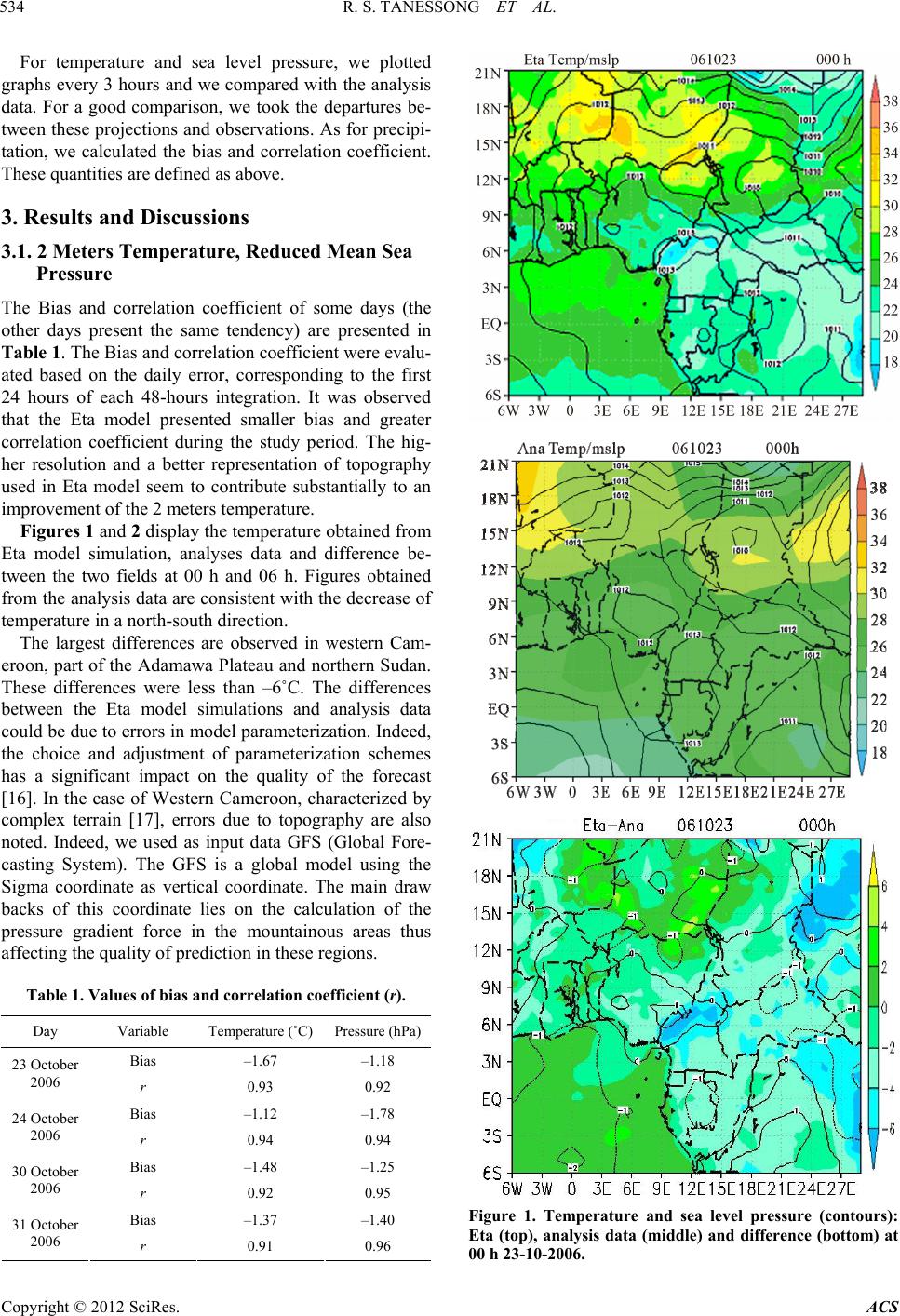

R. S. TANESSONG ET AL.

534

For temperature and sea level pressure, we plotted

graphs every 3 hours and we compared with the analysis

data. For a good comparison, we took the departures be-

tween these projections and observations. As for precipi-

tation, we calculated the bias and correlation coefficient.

These quantities are defined as above.

3. Results and Discussions

3.1. 2 Meters Temperature, Reduced Mean Sea

Pressure

The Bias and correlation coefficient of some days (the

other days present the same tendency) are presented in

Table 1. The Bias and correlation coefficient were evalu-

ated based on the daily error, corresponding to the first

24 hours of each 48-hours integration. It was observed

that the Eta model presented smaller bias and greater

correlation coefficient during the study period. The hig-

her resolution and a better representation of topography

used in Eta model seem to contribute substantially to an

improvement of the 2 meters temperature.

Figures 1 and 2 display the temperature obtained from

Eta model simulation, analyses data and difference be-

tween the two fields at 00 h and 06 h. Figures obtained

from the analysis data are consistent with the decrease of

temperature in a north-south direction.

The largest differences are observed in western Cam-

eroon, part of the Adamawa Plateau and northern Sudan.

These differences were less than –6˚C. The differences

between the Eta model simulations and analysis data

could be due to errors in model parameterization. Indeed,

the choice and adjustment of parameterization schemes

has a significant impact on the quality of the forecast

[16]. In the case of Western Cameroon, characterized by

complex terrain [17], errors due to topography are also

noted. Indeed, we used as input data GFS (Global Fore-

casting System). The GFS is a global model using the

Sigma coordinate as vertical coordinate. The main draw

backs of this coordinate lies on the calculation of the

pressure gradient force in the mountainous areas thus

affecting the quality of prediction in these regions.

Table 1. Values of bias and correlation coefficient (r).

Day Variable Temperature (˚C) Pressure (hPa)

Bias –1.67 –1.18

23 October

2006 r 0.93 0.92

Bias –1.12 –1.78

24 October

2006 r 0.94 0.94

Bias –1.48 –1.25

30 October

2006 r 0.92 0.95

Bias –1.37 –1.40

31 October

2006 r 0.91 0.96

Figure 1. Temperature and sea level pressure (contours):

Eta (top), analysis data (middle) and difference (bottom) at

00 h 23-10-2006.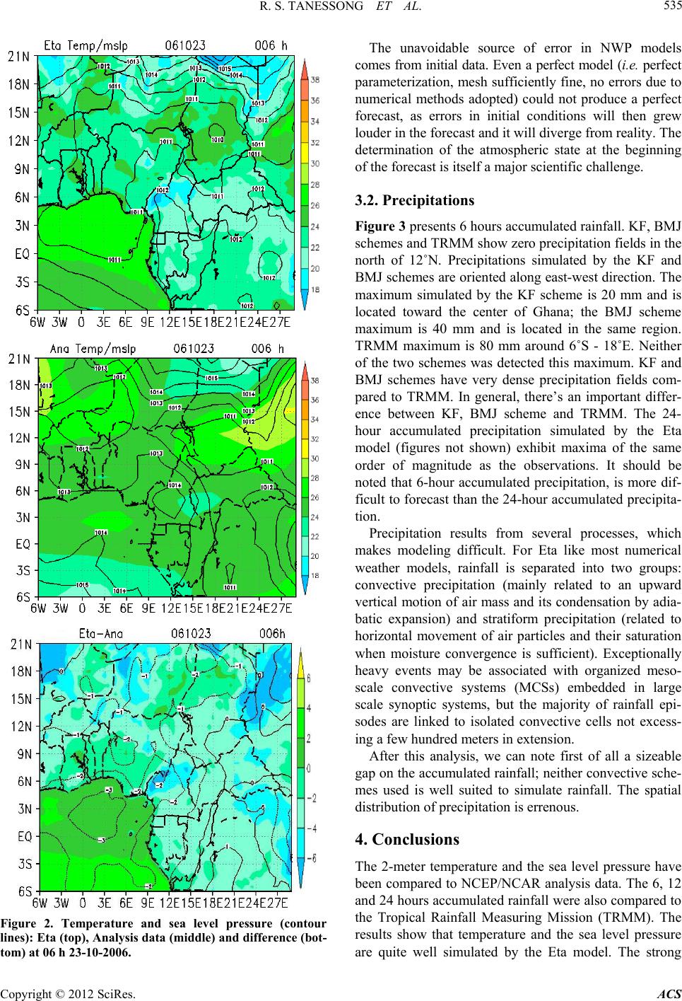

R. S. TANESSONG ET AL. 535

Figure 2. Temperature and sea level pressure (contour

lines): Eta (top), Analysis data (middle) and difference (bot-

tom) at 06 h 23-10-2006.

The unavoidable source of error in NWP models

comes from initial data. Even a perfect model (i.e. perfect

parameterization, mesh sufficiently fine, no errors due to

numerical methods adopted) could not produce a perfect

forecast, as errors in initial conditions will then grew

louder in the forecast and it will diverge from reality. The

determination of the atmospheric state at the beginning

of the forecast is itself a major scientific challenge.

3.2. Precipitations

Figure 3 presents 6 hours accumulated rainfall. KF, BMJ

schemes and TRMM show zero precipitation fields in the

north of 12˚N. Precipitations simulated by the KF and

BMJ schemes are oriented along east-west direction. The

maximum simulated by the KF scheme is 20 mm and is

located toward the center of Ghana; the BMJ scheme

maximum is 40 mm and is located in the same region.

TRMM maximum is 80 mm around 6˚S - 18˚E. Neither

of the two schemes was detected this maximum. KF and

BMJ schemes have very dense precipitation fields com-

pared to TRMM. In general, there’s an important differ-

ence between KF, BMJ scheme and TRMM. The 24-

hour accumulated precipitation simulated by the Eta

model (figures not shown) exhibit maxima of the same

order of magnitude as the observations. It should be

noted that 6-hour accumulated precipitation, is more dif-

ficult to forecast than the 24-hour accumulated precipita-

tion.

Precipitation results from several processes, which

makes modeling difficult. For Eta like most numerical

weather models, rainfall is separated into two groups:

convective precipitation (mainly related to an upward

vertical motion of air mass and its condensation by adia-

batic expansion) and stratiform precipitation (related to

horizontal movement of air particles and their saturation

when moisture convergence is sufficient). Exceptionally

heavy events may be associated with organized meso-

scale convective systems (MCSs) embedded in large

scale synoptic systems, but the majority of rainfall epi-

sodes are linked to isolated convective cells not excess-

ing a few hundred meters in extension.

After this analysis, we can note first of all a sizeable

gap on the accumulated rainfall; neither convective sche-

mes used is well suited to simulate rainfall. The spatial

distribution of precipitation is errenous.

4. Conclusions

The 2-meter temperature and the sea level pressure have

been compared to NCEP/NCAR analysis data. The 6, 12

and 24 hours accumulated rainfall were also compared to

the Tropical Rainfall Measuring Mission (TRMM). The

results show that temperature and the sea level pressure

are quite well simulated by the Eta model. The strong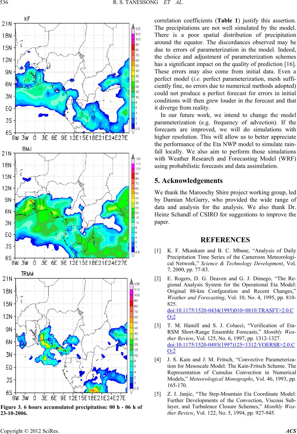

R. S. TANESSONG ET AL.

536

Figure 3. 6 hours accumulated precipitation: 00 h - 06 h of

23-10-2006.

correlation coefficients (Table 1) justify this assertion.

The precipitations are not well simulated by the model.

There is a poor spatial distribution of precipitation

around the equator. The discordances observed may be

due to errors of parameterization in the model. Indeed,

the choice and adjustment of parameterization schemes

has a significant impact on the quality of prediction [16].

These errors may also come from initial data. Even a

perfect model (i.e. perfect parameterization, mesh suffi-

ciently fine, no errors due to numerical methods adopted)

could not produce a perfect forecast for errors in initial

conditions will then grew louder in the forecast and that

it diverge from reality.

In our future work, we intend to change the model

parameterization (e.g. frequency of advection). If the

forecasts are improved, we will do simulations with

higher resolution. This will allow us to better appreciate

the performance of the Eta NWP model to simulate rain-

fall locally. We also aim to perform those simulations

with Weather Research and Forecasting Model (WRF)

using probabilistic forecasts and data assimilation.

5. Acknowledgements

We thank the Maroochy Shire project working group, led

by Damian McGarry, who provided the wide range of

data and analysis for the analysis. We also thank Dr.

Heinz Schandl of CSIRO for suggestions to improve the

paper.

REFERENCES

[1] K. F. Mkankam and B. C. Mbane, “Analysis of Daily

Precipitation Time Series of the Cameroon Meteorologi-

cal Network,” Science & Technology Development, Vol.

7, 2000, pp. 77-83.

[2] E. Rogers, D. G. Deaven and G. J. Dimego, “The Re-

gional Analysis System for the Operational Eta Model:

Original 80-km Confguration and Recent Changes,”

Weather and Forecasting, Vol. 10, No. 4, 1995, pp. 810-

825.

doi:10.1175/1520-0434(1995)010<0810:TRASFT>2.0.C

O;2

[3] T. M. Hamill and S. J. Colucci, “Verification of Eta-

RSM Short-Range Ensemble Forecasts,” Monthly Wea-

ther Review, Vol. 125, No. 6, 1997, pp. 1312-1327.

doi:10.1175/1520-0493(1997)125<1312:VOERSR>2.0.C

O;2

[4] J. S. Kain and J. M. Fritsch, “Convective Parameteriza-

tion for Mesoscale Model: The Kain-Fritsch Scheme. The

Representation of Cumulus Convection in Numerical

Models,” Meteorological Monographs, Vol. 46, 1993, pp.

165-170.

[5] Z. I. Janjic, “The Step-Mountain Eta Coordinate Model:

Further Developments of the Convection, Viscous Sub-

layer, and Turbulence Closure Schemes,” Monthly Wea-

ther Review, Vol. 122, No. 5, 1994, pp. 927-945.

R. S. TANESSONG ET AL.

537

doi:10.1175/1520-0493(1994)122<0927:TSMECM>2.0.

CO;2

[6] T. Black, “The NMC Mesoscale Eta Model: Description

and Forecast Examples,” Weather and Forecasting, Vol.

9, No. 2, 1994, pp. 265-278.

doi:10.1175/1520-0434(1994)009<0265:TNNMEM>2.0.

CO;2

[7] S. C. Chou, J. F. B. Fonseca and J. L. Gomes, “Evalua-

tion of Eta Model Seasonal Precipitation Forecasts over

South America,” Nonlinear Processes in Geophysics, Vol.

12, No. 4, 2005, pp. 537-555.

doi:10.5194/npg-12-537-2005

[8] M. J. Fennessy and J. Shukla, “Seasonal Prediction over

North America with a Regional Model Nested in a Global

Model,” Journal of Climate, Vol. 13, No. 14, 2000, pp.

2605-2627.

doi:10.1175/1520-0442(2000)013<2605:SPONAW>2.0.

CO;2

[9] F. Mesinger, Z. I. Janjic, S. Nickovic, D. Gavrilov and D.

G. Deaven, “The Step-Mountain Coordinate: Model De-

scription and Performance for Cases of Alpine Lee Cyc-

logenesis and for a Case of an Appalachian Redevelop-

ment,” Monthly Weather Review, Vol. 116, No. 7, 1988,

pp. 1493-1518.

doi:10.1175/1520-0493(1988)116<1493:TSMCMD>2.0.

CO;2

[10] F. Mesinger, “A Blocking Technique for Representation

of Mountains in Atmospheric Models,” Avition Meteoro-

logical Aeronautics, Vol. 44, 1984, pp. 195-202.

[11] G. L. Mellor and T. Yamada, “Development of a Turbu-

lence Closure Model for Geophysical Fluid Problems,”

Reviews of Geophysics and Space Physics, Vol. 20, No. 4,

1974, pp. 851-875. doi:10.1029/RG020i004p00851

[12] S. B. Fels and M. D. Schawarztkopf, “The Simplified

Exchange Approximation: A New Method for Radiative

Transfer Calculations,” Journal of the Atmospheric Sci-

ences, Vol. 32, No. 7, 1975, pp. 1475-1488.

doi:10.1175/1520-0469(1975)032<1475:TSEAAN>2.0.C

O;2

[13] A. A. Lacis and J. E. Hansen, “A Parametrization of the

Absorption Dissipation in the Atmosphere from Large-

Scale Balance Requirements,” Monthly Weather Review,

Vol. 49, 1975, pp. 608-627.

[14] W. A. J. Gallus and M. Segal, “Does Increased Predicted

Warm Season Rainfall Indicate Enhanced Likelihood of

Rain Occurrence?” Weather and Forecasting, Vol. 19, No.

6, 2004, pp. 1127-1135. doi:10.1175/820.1

[15] S. E. Nicholson, B. Some, J. McCollum, E. Nelkin, D.

Klotter, Y. Berte, B. M. Diallo, I. Gaye, G. Kpabeba, O.

Ndiaye, J. N. Noukpozounkou, M. M. Tanu, A. Thiam, A.

A. Toure and A. K. Traore, “Validation of TRMM and

Other Rainfall Estimates with a High-Density Gauge

Dataset for West Africa. Part II: Validation of TRMM

Rainfall Products,” Journal of Applied Meteorology, Vol.

42, No. 10, 2003, pp. 1355-1368.

[16] J. Venkata Ratnam and J. Krishna Kumar, “Sensitivity of

the Simulated Monsoons of 1987 and 1988 to Convective

Parameterization Schemes in MM5,” Journal of Climate,

Vol. 18, 2005, pp. 2724-2741.

[17] E. Richard, A. Buzzi and G. Zangl, “Quantitative Pre-

cipitation Forecasting in the Alps: The Advances Achie-

ved by the Mesoscale Alpine Programme,” Quarterly

Journal of the Royal Meteorological Society, Vol. 133,

2007, pp. 831-846.