

Paper Menu >>
Journal Menu >>
 Theoretical Economics Letters, 2012, 2, 408-411 http://dx.doi.org/10.4236/tel.2012.24075 Published Online October 2012 (http://www.SciRP.org/journal/tel) Further Results on Convergence for Nonlinear Transformations of Fractionally Integrated Time Series Chien-Ho Wang Department of Economics, National Taipei University, New Taipei City, Chinese Taipei Email: [email protected] Received May 6, 2012; revised June 4, 2012; accepted July 2, 2012 ABSTRACT This paper presents some new results for the nonlinear tran sformations of the fractional integration process. Specifically, this paper reviews the weight fractional integration process with the Hurst parameter, 32> >56d, and investigates the asymptotics of asymptotically homogeneous functional transformations of weight fractional integration process. These new results improve upon the earlier research of Tyurin and Phillips [1]. Keywords: Long Memory; Fractional Brownian Motion; Tanaka Formula; Nonlinearity 1. Introduction Since the breakthrough papers of Park and Phillips [2, 3 ], the research on the nonlin ear cointegration has generated a lot of interest in recent years. In traditional research on cointegration, econometricians always adopt linear models. Using a linear cointegration model, econometricians can derive large sample properties easily. However, these settings have a serious drawback: there are many non- linear relationships between dependent variables and independent v ariables in the cointegration mo del. Thus, it is a subjective process to set cointegration as a linear form in advance. A nonlinear regression model may improve this problem in a cointegration system. Although nonlinear regressions have obvious merit for cointe- gration models, it is difficult to derive the asymptotics for their estimated parameters and test statistics. Park and Phillips [2, 3] were the first to use local time to obtain asymptotics under nonlinear transformations of the I(1) process. Pötscher [4] and de Jong and Wang [5] later extended to these results to more flexible assumptions. The asymptotics of nonlinear transformations for non- stationary time series consistently concentrated on the I(1) process in early nonlinear cointegration research. Tyurin and Phillips [1] extended their method to the nonsta- tionary I(d) process. Jeganathan [6] investigated the asy- mptotics of nonlinear transformations for generalized fractional stable motions. Although they presented some new results for the nonlinear transformations of the non- stationary fractionally integrated process, they only con- centrated on integrable functions. This paper uses a weight nonstationary fractionally integrated process instead of the standard nonstationary fractionally integrated process. This paper extends the results of Tyurin and Phillips [1] to asymptotically homogeneous functions. Specifically, this paper uses the fractional Brownian motion Tanaka formula to obtain the asymptotics of nonlinear transformations for the non- stationary fractional integration process. The results of this paper address the shortcomings of Tyurin and Phillips [1]. 2. Assumptions and Basic Results Consider the following fractional integration processes: 1= d t Lx t (1) where t is an 2 ... 0,iid and 32> >56d. t is called a nonstationary fractionally integrated processes. In addition to the definition of nonstationary fractionally integrated processes, This paper uses the following ad- ditional assumptions. x Assumption 1. For some >2>2max1,2qp H, < q k E and 2< t E ,where H is the Hurst exponent, =12,and 2Hd p Assumpti on 2. 1) 2 =1 = nH t t VarxnM n , where M n is a slowly varying function. 2) The distribution of k , , is abso- lutely continuous with respect to the Lebesgue measure and has characteristic function for which =0, 1,2,k =it k tEe =0 limttt for some >0 . Based on these assumptions, we can obtain the frac- tional central limit theorem for the nonstationary I(d) p ro- cesses. Theorem 1. Consider the process defined by C opyright © 2012 SciRes. TEL 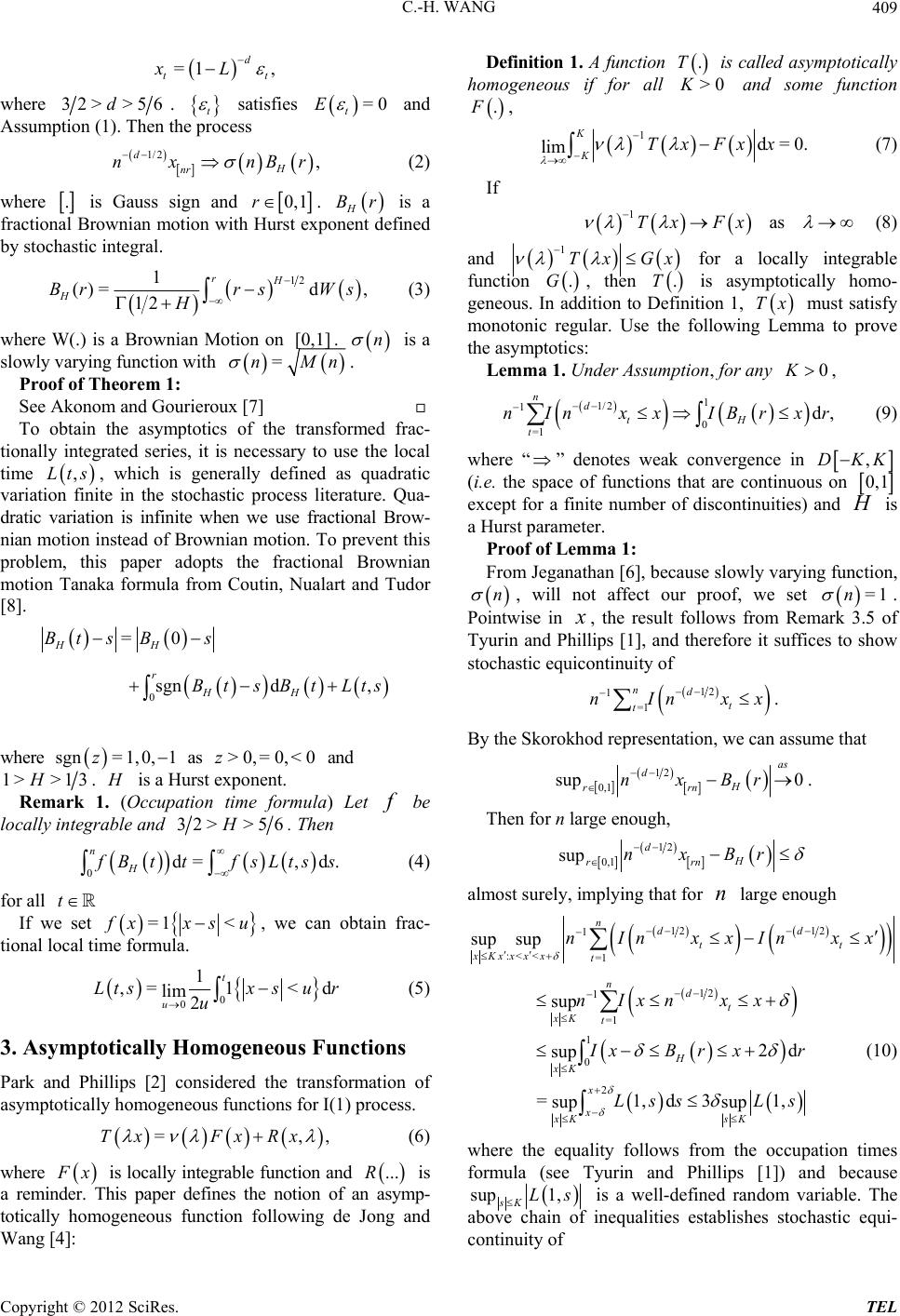 C.-H. WANG 409 =1 , d tt xL where 32> >56d. t satisfies and Assumption (1). Then the process =0 t E 1/2, dH nr nx nBr (2) where . is Gauss sign and 0,1r. H Br is a fractional Brownian motion with Hurst exponent defined by stochastic integral. 12 1 ()=d , 12 rH H Brrs Ws H (3) where W(.) is a Brownian Motion on . [0,1] n is a slowly varying function with =nMn konurie7] o obtain the asymptotics of the transformed frac- tio . Proof of Theorem 1: See Aom and Goroux [ T nally integrated series, it is necessary to use the local time ,Lts, which is generally defined as quadratic variatte in the stochastic process literature. Qua- dratic variation is infinite when we use fractional Brow- nian motion instead of Brownian motion. To prevent this problem, this paper adopts the fractional Brownian motion Tanaka formula from Coutin, Nualart and Tudor [8]. ion fini 0 =0 sgnd, HH r HH Bt sBs Bt sBtLts where as and sgn=1,0, 1z>0,=0,<0z 1> >H13. H is a Hurst exponent. Remark ula) Let be lo 1Occupation time form. (f cally integrable and 32> >56H. Then n 0d=, d. H f Bt tfsLtss (4) for all e set t If w =1 < f xxs ula. u , we can obtain frac- tional local time form 0 0 1 ,=1 <d lim 2 t u Ltsx sur u (5) 3. Asymptotically Homogeneous Functions of Park and Phillips [2] considered the transformation asymptotically homogeneous functions for I(1) process. =,,Tx FxRx (6) where F x is locally integrable function and ...R is a reminder. This paper defines the notion of an asymp- totically homogeneous function following de Jong and Wang [4]: Definition 1. A function is called asymptotically ho .T>K mogeneous if for all 0 and some function . F , 1d=0. lim K KTxFxx (7) If (8) and 1asTx Fx 1Tx Gx for a locally integrable ion funct .G, then .T is asymptotically homo- geneous. ition to Definition 1, Tx must satisfy monotonic regular. Use the followingma to prove the asymptotics: Lemma 1. Und In add Lem er Assumption, for any (9) where “” denotes weak convergence in 0K, 1 1/2 nd 1 nIn 0 =1 d, tH t xx IBrxr ,DKK on (i.e. the space of functions that are continuous 0,1 except for a finite number of discontinuities) and H is a Hurst parameter. Proof of Lemma 1: because slowly varying function, From Jeganathan [6], n, will not affect our proof, we set =1n . ise in Pointw x , the result follows from Remf Tyurin and Phlips [1], and therefore it suffices to show stochastic equicontinuity of ark 3.5 o il 12 =1 t txx. By the Skorokhod representation, we can assume that 1nd nIn 12 as d 0,1 0 sup H rrn nxBr . Then for n large enough, 12 sup d nx 0,1H rrn Br almost surely, implying that for large enough n 12 12 1 :< <=1 sup supndd tt xKxxxx t nInxxInxx 12 1 =1 1 0 2 sup 2d sup =1,d3 sup sup ndt xK t H xK x x xK sK nIxn xx 1, I xBrx LssLs r (10) where the equality follows from the occupation times formula (see Tyurin and Phillips [1]) and because 1, sup sK Ls is a well-defined random variable. The above chain of inequalities establishes stochastic equi- continuity of Copyright © 2012 SciRes. TEL 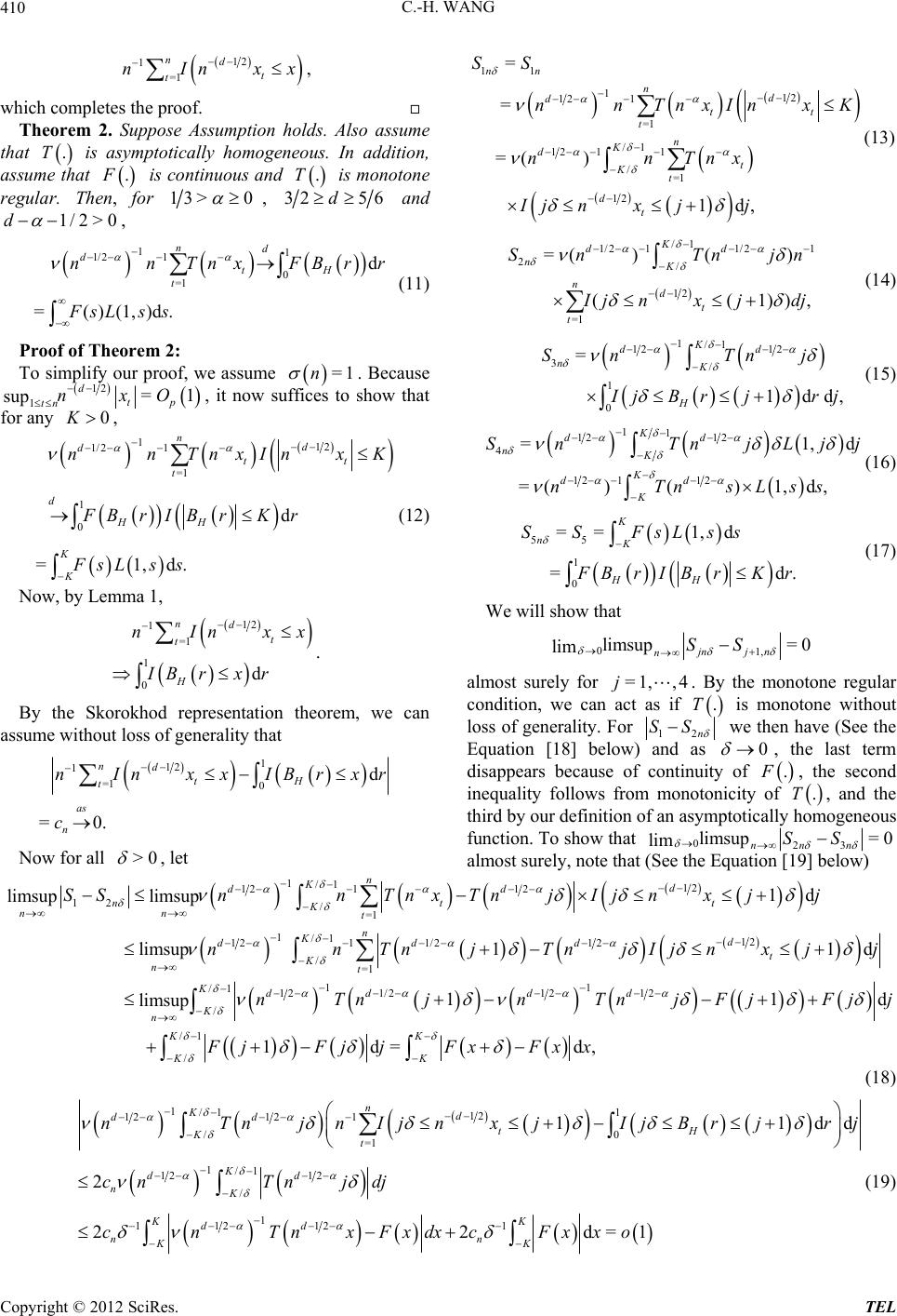 C.-H. WANG Copyright © 2012 SciRes. TEL 410 12 1 =1 ndt t nInxx , 11 112 12 1 =1 /1 12 11 /=1 12 = = =() 1d, nn nd dtt t n K dt Kt dt SS nnTnxInx nnTnx Ij nxjj K (13) w hich completes the proof. Theorem 2. Suppose Assumption holds. Also assume that .T is asymptotically homogeneous. In additio as n, sume that . F is continuous and .T is monotone regular. Then, for 13> 0 , 32 56d and 1/2>d0 11d d , /1 1/211/21 2/ 12 =1 =( )() ((1)), K dd nK ndt t Sn Tnjn I jnx jdj (14) 1 1/2 0 =1 d =()(1,)d. n tH t nnTnxFBr FsLs s r (11) Proof of Theorem 2: To simplify our proof, we assume. Because 1/1 12 12 3/ 1 0 = 1dd, K dd nK H Sn Tnj I jBr jrj (15) =1n 12 1=1 pdtp tn nxO su , it now sufat fo fices to show th r any 0K, 11 12 12 4 12 112 =1 =()()1,d, K dd nK K dd K Sn TnjLj nTnsLs 1 1/21 =1 1 0 d =1,d. n d t d HH K K nnT FBrI BrKr FsLs s (12) Now, by Lemma 1, ,dj s (16) 12 d tt nxInxK 55 1 0 == 1,d =d. K nK HH SS FsLss F BrIBr Kr (17) We will show that 12 1 =1 1 0 d ndt t nI H nxx IBrx r . By the Skorokhod representation theorem, we can assume without loss of generality that 01, =0 lims u p lim jnj n nSS almost surely for . By the monotone regular condition, we can act as if is monotone without loss of generality. For =1, ,4j .T 12n SS we then have (See the Equation [18] below) and as 0 , the last term disappears because of continuity of . F , the second inequality follows from monotonicity of .T, and the third by our definition of a n as ymptotically homogeneous function. To show that 0lims lim 1 12 1 =1 0 d ndtH t nInxxIBrxr =0 . as n c Now for all 23 =0 nn SS upn almost surely, note that (See the Equation [19] below) >0 , let 1/1 12 12 112 12 msup msup nt nn SS /=1 1/1 12 12 1 1/212 /=1 1d li li 11d limsup n Kd dd t Kt n Kd dddt K nt nnTnx TnjIjnxjj nnTnjTnjIjnxjj 11 /1 12 1/212 12 / /1 / 11d limsup 1d=d, Kdd dd K n KK KK nTnjnTnjFjFjj FjFjjFxFxx (18) 1/1 1 12 1212 1 / 0 =1 1/1 12 12 / 1 112 121 11 2 22d=1 n Kd dd tH Kt K dd nK KK dd n n KK nTnjnIjnxjIjBrj cnTn jdj cnTnxFxdxcFxxo ddrj (19) 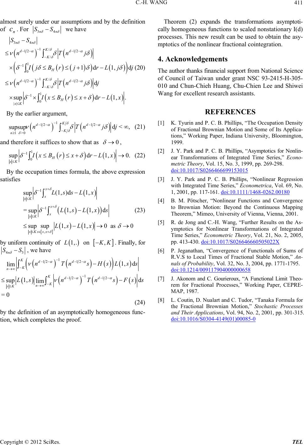 C.-H. WANG 411 almost surely under our assumptions and by the definition of . For n c34nn SS we have 34 1/ 12 12 / 1 1 0 / 1 1 0 || 1d1,d d1,. sup nn K dd K H K H xK SS nTnj I 1/ 12 12 d K dd jBrjrLj j IxBrxrLx (20) By the earlier argument, nT njj 1 12 12 1>0 d< , supsup K dd K nnTnj j and therefore it suffices to show that as (21) 0 , 1 1 0d1, sup H xK IxBrxr Lx 0. (22) ormula, the above expressi satisfies By the occupation times fon 1 1 (1, )d1, sup =1,1,d sup x x xK LssLx LsLxs continuity of on ,1, 1,0as0 sup sup xK sxxLsLx by uniform x xK x (23) 1,.L , K K. Finally, for 45n SS , we have 1 12 12 1 12 12 1,d lim 1, d sup lim =0 Kdd K n Kdd K n sK nTnsHsLs LsnTn sFss s by the defiptotically homogeneous fu nc- tion, which completes th e proof. Theorem (2) expands the transformations asymptoti- cally homogeneous functions to scaled nonstationary I(d) processes. This new result can be used to obtain the asy- mptotics of the nonlinear fractional cointegration. 4. Acknowledgements The author thanks financial support from National Science NCES [2] J. Y. Park and P. C. B. Phillips, “Asymptotics for Nonlin- ear Transforme Series,” Econo- metric Theory. 269-298. (24) nition of an asym of Council of Taiwan under grant NSC 93-2415-H-305- 010 and Chun-Chieh Huang, Chu-Chien Lee and Shiwei Wang for excellent research assistants. REFERE [1] K. Tyurin and P. C. B. Phillips, “The Occupation Density of Fractional Brownian Motion and Some of Its Applica- tions,” Working Paper, Indiana University, Bloomington, 1999. ations of Integrated Tim , Vol. 15, No. 3, 1999, pp doi:10.1017/S0266466699153015 [3] J. Y. Park and P. C. B. Phillips, “Nonlinear Regression with Integrated Time Series,” Econometrica, Vol. 69, No. 1, 2001, pp. 117-161. doi:10.1111/1468-0262.00180 [4] B. M. Pötscher, “Nonlinear Functions and Convergence to Brownian Motion: Beyond the Continuous Mapping Theorem,” Mimeo, University of Vienna, Vienna, 20 [5] R. de Jong and C.-H. Wang, “Furt 01. her Results on the As- ymptotics for Nonlinear Transformations of Integrated Time Series,” Econometric Theory, Vol. 21, No. 2, 2005, pp. 413-430. doi:10.1017/S026646660505022X [6] P. Jeganathan, “Convergence of Functionals of Sums of R.V.S to Local Times of Fractional Stable Motion,” An- nals of Probability, Vol. 32, No. 3, 2004, pp. 1771-1795. doi:10.1214/009117904000000658 [7] J. Akonom and C. Gourieroux, “A Functional Limit Theo- rem for Fractional Processes,” Working Paper, CEPRE- MAP, 1987. [8] L. Coutin, D. Nualart and C. Tudor, “Tanaka Formula for the Fractional Brownian Motion,” Stochastic Processes and Their Applications, Vol. 94, No. 2, 2001, pp. 301-315. doi:10.1016/S0304-4149(01)00085-0 Copyright © 2012 SciRes. TEL |