Generalization of the Second Order Vector Potential Formulation for Arbitrary Non-Orthogonal Curvilinear Coordinates Systems from the Covariant Form of Maxwell's Equations

doi:10.4236/jemaa.2012.410055

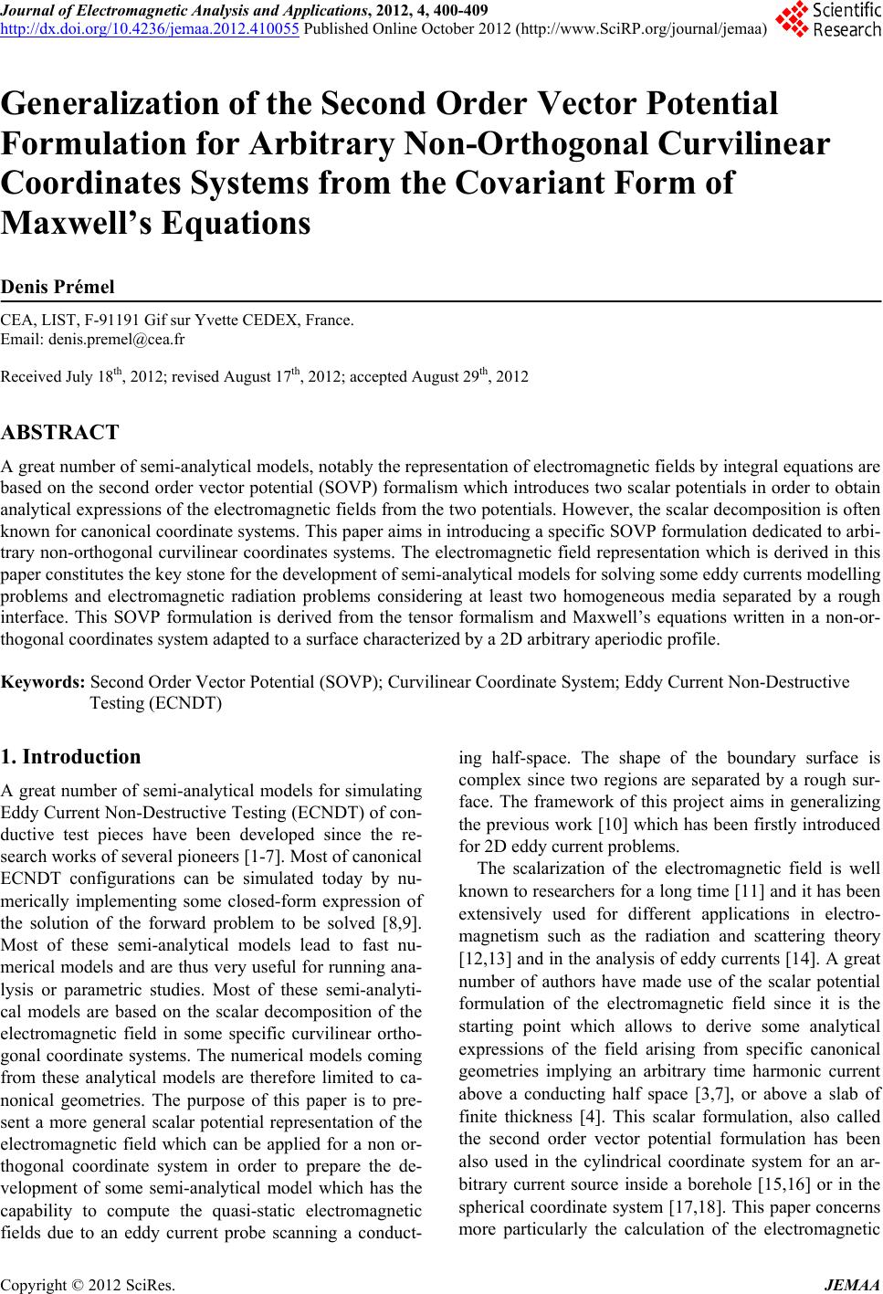Journal of Electromagnetic Analysis and Applications, 2012, 4, 400-409

http://dx.doi.org/10.4236/jemaa.2012.410055 Published Online October 2012 (http://www.SciRP.org/journal/jemaa)

Generalization of the Second Order Vector Potential

Formulation for Arbitrary Non-Orthogonal Curvilinear

Coordinates Systems from the Covariant Form of

Maxwell’s Equations

Denis Prémel

CEA, LIST, F-91191 Gif sur Yvette CEDEX, France.

Email: denis.[email protected]

Received July 18th, 2012; revised August 17th, 2012; accepted August 29th, 2012

ABSTRACT

A great number of semi-analytical models, notably the representation of electromagnetic fields by integral equations are

based on the second order vector potential (SOVP) formalism which introduces two scalar potentials in order to obtain

analytical expressions of the electromagnetic fields from the two potentials. However, the scalar decomposition is often

known for canonical coordinate systems. This paper aims in introducing a specific SOVP formulation dedicated to arbi-

trary non-orthogonal curvilinear coordinates systems. The electromagnetic field representation which is derived in this

paper constitutes the key stone for the development of semi-analytical models for solving some eddy currents modelling

problems and electromagnetic radiation problems considering at least two homogeneous media separated by a rough

interface. This SOVP formulation is derived from the tensor formalism and Maxwell’s equations written in a non-or-

thogonal coordinates system adapted to a surface characterized by a 2D arbitrary aperiodic profile.

Keywords: Second Order Vector Potential (SOVP); Curvilinear Coordinate System; Eddy Current Non-Destructive

Testing (ECNDT)

1. Introduction

A great number of semi-analytical models for simulating

Eddy Current Non-Destructive Testing (ECNDT) of con-

ductive test pieces have been developed since the re-

search works of several pioneers [1-7]. Most of canonical

ECNDT configurations can be simulated today by nu-

merically implementing some closed-form expression of

the solution of the forward problem to be solved [8,9].

Most of these semi-analytical models lead to fast nu-

merical models and are thus very useful for running ana-

lysis or parametric studies. Most of these semi-analyti-

cal models are based on the scalar decomposition of the

electromagnetic field in some specific curvilinear ortho-

gonal coordinate systems. The numerical models coming

from these analytical models are therefore limited to ca-

nonical geometries. The purpose of this paper is to pre-

sent a more general scalar potential representation of the

electromagnetic field which can be applied for a non or-

thogonal coordinate system in order to prepare the de-

velopment of some semi-analytical model which has the

capability to compute the quasi-static electromagnetic

fields due to an eddy current probe scanning a conduct-

ing half-space. The shape of the boundary surface is

complex since two regions are separated by a rough sur-

face. The framework of this project aims in generalizing

the previous work [10] which has been firstly introduced

for 2D eddy current problems.

The scalarization of the electromagnetic field is well

known to researchers for a long time [11] and it has been

extensively used for different applications in electro-

magnetism such as the radiation and scattering theory

[12,13] and in the analysis of eddy currents [14]. A great

number of authors have made use of the scalar potential

formulation of the electromagnetic field since it is the

starting point which allows to derive some analytical

expressions of the field arising from specific canonical

geometries implying an arbitrary time harmonic current

above a conducting half space [3,7], or above a slab of

finite thickness [4]. This scalar formulation, also called

the second order vector potential formulation has been

also used in the cylindrical coordinate system for an ar-

bitrary current source inside a borehole [15,16] or in the

spherical coordinate system [17,18]. This paper concerns

more particularly the calculation of the electromagnetic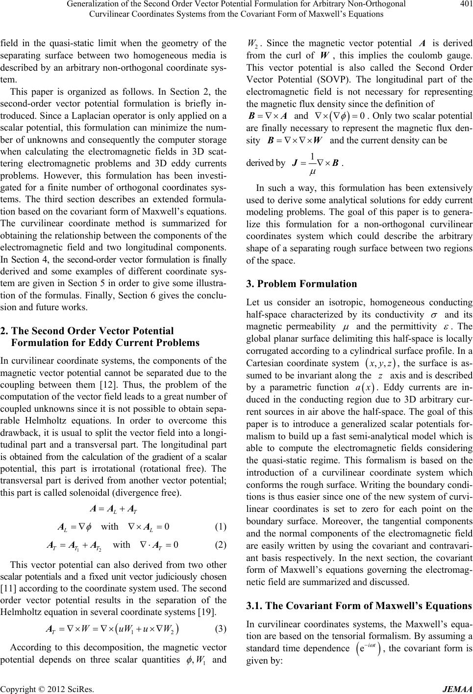

Generalization of the Second Order Vector Potential Formulation for Arbitrary Non-Orthogonal

Curvilinear Coordinates Systems from the Covariant Form of Maxwell’s Equations

401

field in the quasi-static limit when the geometry of the

separating surface between two homogeneous media is

described by an arbitrary non-orthogonal coordinate sys-

tem.

This paper is organized as follows. In Section 2, the

second-order vector potential formulation is briefly in-

troduced. Since a Laplacian operator is only applied on a

scalar potential, this formulation can minimize the num-

ber of unknowns and consequently the computer storage

when calculating the electromagnetic fields in 3D scat-

tering electromagnetic problems and 3D eddy currents

problems. However, this formulation has been investi-

gated for a finite number of orthogonal coordinates sys-

tems. The third section describes an extended formula-

tion based on the covariant form of Maxwell’s equations.

The curvilinear coordinate method is summarized for

obtaining the relationship between the components of the

electromagnetic field and two longitudinal components.

In Section 4, the second-order vector formulation is finally

derived and some examples of different coordinate sys-

tem are given in Section 5 in order to give some illustra-

tion of the formulas. Finally, Section 6 gives the conclu-

sion and future works.

2. The Second Order Vector Potential

Formulation for Eddy Current Problems

In curvilinear coordinate systems, the components of the

magnetic vector potential cannot be separated due to the

coupling between them [12]. Thus, the problem of the

computation of the vector field leads to a great number of

coupled unknowns since it is not possible to obtain sepa-

rable Helmholtz equations. In order to overcome this

drawback, it is usual to split the vector field into a longi-

tudinal part and a transversal part. The longitudinal part

is obtained from the calculation of the gradient of a scalar

potential, this part is irrotational (rotational free). The

transversal part is derived from another vector potential;

this part is called solenoidal (divergence free).

L

T

AA A

with 0

LL



 AA

2

(1)

12

with 0

TTT T

 AAAA (2)

This vector potential can also derived from two other

scalar potentials and a fixed unit vector judiciously chosen

[11] according to the coordinate system used. The second

order vector potential results in the separation of the

Helmholtz equation in several coordinate systems [19].



1TWuWuW A (3)

According to this decomposition, the magnetic vector

potential depends on three scalar quantities 1

,W



and

2. Since the magnetic vector potential W

A

is derived

from the curl of W, this implies the coulomb gauge.

This vector potential is also called the Second Order

Vector Potential (SOVP). The longitudinal part of the

electromagnetic field is not necessary for representing

the magnetic flux density since the definition of





B

A and





0





 . Only two scalar potential

are finally necessary to represent the magnetic flux den-

sity





B

W and the current density can be

derived by 1







J

B.

In such a way, this formulation has been extensively

used to derive some analytical solutions for eddy current

modeling problems. The goal of this paper is to genera-

lize this formulation for a non-orthogonal curvilinear

coordinates system which could describe the arbitrary

shape of a separating rough surface between two regions

of the space.

3. Problem Formulation

Let us consider an isotropic, homogeneous conducting

half-space characterized by its conductivity



and its

magnetic permeability



and the permittivity



. The

global planar surface delimiting this half-space is locally

corrugated according to a cylindrical surface profile. In a

Cartesian coordinate system



,,



x

yz

z



, the surface is as-

sumed to be invariant along the axis and is described

by a parametric function . Eddy currents are in-

duced in the conducting region due to 3D arbitrary cur-

rent sources in air above the half-space. The goal of this

paper is to introduce a generalized scalar potentials for-

malism to build up a fast semi-analytical model which is

able to compute the electromagnetic fields considering

the quasi-static regime. This formalism is based on the

introduction of a curvilinear coordinate system which

conforms the rough surface. Writing the boundary condi-

tions is thus easier since one of the new system of curvi-

linear coordinates is set to zero for each point on the

boundary surface. Moreover, the tangential components

and the normal components of the electromagnetic field

are easily written by using the covariant and contravari-

ant basis respectively. In the next section, the covariant

form of Maxwell’s equations governing the electromag-

netic field are summarized and discussed.



ax

3.1. The Covariant Form of Maxwell’s Equations

In curvilinear coordinates systems, the Maxwell’s equa-

tion are based on the tensorial formalism. By assuming a

standard time dependence





it



e, the covariant form is

given by: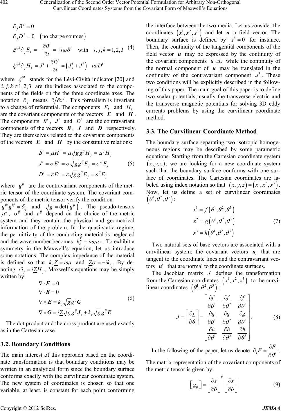

Generalization of the Second Order Vector Potential Formulation for Arbitrary Non-Orthogonal

Curvilinear Coordinates Systems from the Covariant Form of Maxwell’s Equations

402



0

0no charge sources

with,,1, 2,3

j

i

ijk i

jk

i

ijkii ii

jk s

B

D

B

EiBijk

t

D

HJ JJiD

t









 



 





(4)

where ijk



stands for the Lévi-Cività indicator [20] and

are the indices associated to the compo-

nents of the fields on the the three coordinate axes. The

notation

, ,3ijk1, 2,

j

 means

j

x

 . This formalism is invariant

to a change of referential. The components and

k

Ek

H

are the covariant components of the vectors

E

and

H

.

The components ,

i

Bi

J

and are the contravariant

components of the vectors ,

i

D

B

J

and respectively.

They are themselves related to the covariant components

of the vectors

D

E

and

H

by the constitutive relations:

i iijij

j

i iijij

j

i iijij

jj

BHggHH

J

EggEE

DEggE E

 

 

 

 

(5)

where ij

g

are the contravariant components of the met-

ric tensor of the coordinate system. The covariant com-

ponents of the metric tensor verify the condition

ik kj

gg ij



 and



det ij

g

g. The pseudo-tensors

ij



, ij



and ij



depend on the choice of the metric

system and they contain the physical and geometrical

information of the problem. In the quasi-static regime,

the permittivity of the conducting material is neglected

and the wave number becomes 2=

c

ki





. To exhibit a

symmetry in the Maxwell’s equation, let us introduce

some notations. The complex impedance of the material

is defined so that c

kZ





 and c

Z

ik



 . By de-

noting

j

ZHGi, Maxwell’s equations may be simply

written by:

0

ij

c

ij ij

sc

kgg

iZ ggkgg

 

 

 

E

B

EG

GJ E

(6)

The dot product and the cross product are used exactly

as in the Cartesian case.

3.2. Boundary Conditions

The main interest of this approach based on the coordi-

nate transformation is that boundary conditions may be

written in an analytical form since the boundary surface

conforms exactly with the curvilinear coordinate system.

The new system of coordinates is chosen so that one

variable, at least, is constant for each point conforming

the interface between the two media. Let us consider the

coordinates





123

,,

x

xx

u

and let u a field vector. The

boundary surface is defined by for instance.

Then, the continuity of the tangential components of the

field vector may be expressed by the continuity of

the covariant components while the continuity of

the normal component of may be translated in the

continuity of the contravariant component . These

two conditions will be explicitly described in the follow-

ing of this paper. The main goal of this paper is to define

two scalar potentials, usually the transverse electric and

the transverse magnetic potentials for solving 3D eddy

currents problems by using the curvilinear coordinate

method.

30x

21

,uu

u

3

u

3.3. The Curvilinear Coordinate Method

The boundary surface separating two isotropic homoge-

neous regions may be described by some parametric

equations. Starting from the Cartesian coordinate system





,,

x

yz , we are looking for a new coordinate system

such that the boundary surface conforms with one sur-

face of coordinates. The Cartesian coordinates are la-

beled using index notation so that







123

,,, ,

x

yzxxx.

Now, let us define a set of curvilinear coordinates





312

,,





:





23





11

212

312

,,

xf

xg

xh



3















(7)

Two natural sets of base vectors are associated with a

curvilinear system: the covariant vectors i that are

tangent to the coordinate lines and the contravariant vec-

tors that are normal to the coordinate surfaces.

u

i

u

The Jacobian matrix

J

defines the transformation

from the Cartesian coordinates



123

,,



x

xx to the curvi-

linear coordinates





12 3

,,





:

123

.

f

ff

x

ggg

J

hhh































































(8)

In the following of the paper, let us denote ii

F









.

The matrix representation of the covariant components of

the metric tensor is given by:

T

ij

x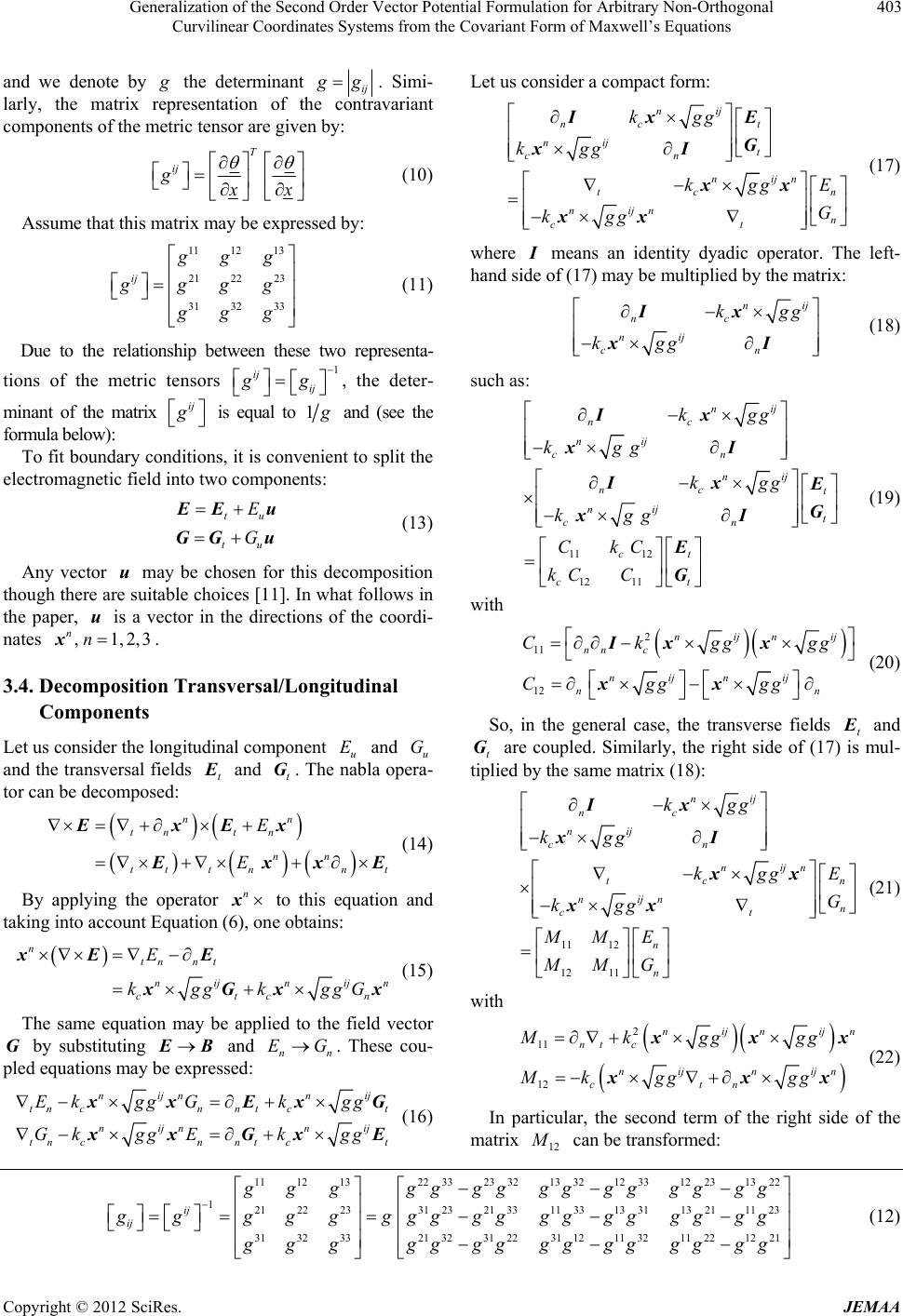

g





 









 







 

(9)

Generalization of the Second Order Vector Potential Formulation for Arbitrary Non-Orthogonal

Curvilinear Coordinates Systems from the Covariant Form of Maxwell’s Equations

403

and we denote by

g

the determinant ij

g

g. Simi-

larly, the matrix representation of the contravariant

components of the metric tensor are given by:

Let us consider a compact form:

nij

nc t

nij t

cn

nijn

tc n

nijn n

ct

kgg

E

G

kgg























 





Ix E

G

xI

xx

(17)

T

ij

g

x











 



(10)

Assume that this matrix may be expressed by:

where means an identity dyadic operator. The left-

hand side of (17) may be multiplied by the matrix:

I

11 12 13

21 22 23

31 32 33

ij

g

gg

g

ggg

g

gg















(11)

ni

nc

nij

cn

kgg

j











 









Ix

xI

(18)

Due to the relationship between these two representa-

tions of the metric tensors , the deter-

1

ij

gg







 such as:

minant of the matrix ij

g





is equal to 1

g

and (see the

formula below):

11 12

12 11

nij

nc

nij

cn

nij

nc t

nij t

cn

ct

kgg

CkC

kC C







 















 











Ix

xI

Ix

E

G

xI

E

G

(19)

To fit boundary conditions, it is convenient to split the

electromagnetic field into two components:

tu

E

G



E

Eu

GG u

(13)

Any vector may be chosen for this decomposition

though there are suitable choices [11]. In what follows in

the paper, is a vector in the directions of the coordi-

nates .

u

,1,

u

n2,

n

x

with





2

11

12

nijnij

nn c

nijnij

nn

Ck gggg

Cgggg





 







 



Ix x

xx

(20)

3

3.4. Decomposition Transversal/Longitudinal

Components So, in the general case, the transverse fields t

E

and

t are coupled. Similarly, the right side of (17) is mul-

tiplied by the same matrix (18):

G

Let us consider the longitudinal component u and u

and the transversal fields

E G

t

E

and . The nabla opera-

tor can be decomposed:

t

G

11 12

12 11

nij

nc

nij

cn

nijn

tc n

nijnn

ct

n

kgg

E

G

kgg

EMM

GMM







 



















 

















Ix

xI

xx

(21)







nn

tntn

nn

ttt nn

E

 

 

ExEx

t

E

xx E

(14)

By applying the operator to this equation and

taking into account Equation (6), one obtains:

nx



n

tn nt

nij nij

ctc

E

kggkggG

  

 

xE E

xGxn

n

x

(15)

with

The same equation may be applied to the field vector

by substituting

G

E

B and . These cou-

pled equations may be expressed:

n

EG







2

11

12

nijnij

nt c

nij nijn

ctn

Mk gggg

M kgggg

 

 

xx

n

x

(22)

n

nijn nij

tn cnntct

nijn nij

tn cnntct

E kggGkgg

GkggEk gg

  

 

xxEx

xxGx

G

E

(16) In particular, the second term of the right side of the

matrix 12

M

can be transformed:

11121322 3323321332123312 2313 22

121222331 23213311 3313 31132111 23

31323321 3231 223112113211 221221

ij

g

gggggggggg gg gg

gggggg gggggggggggg

g

gggggggg gggggg





 





















 





 

(12)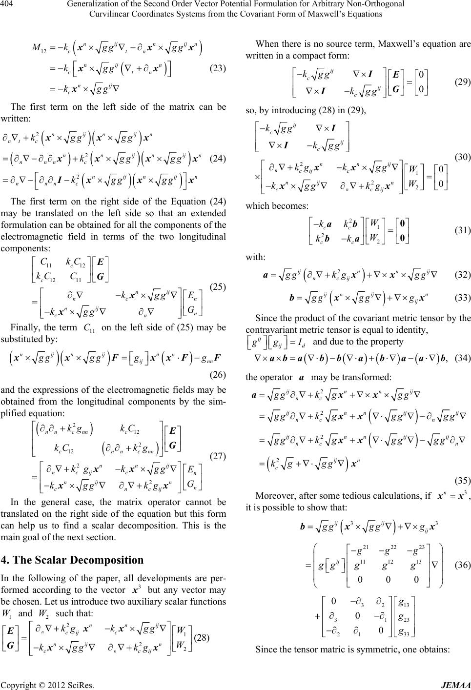

Generalization of the Second Order Vector Potential Formulation for Arbitrary Non-Orthogonal

Curvilinear Coordinates Systems from the Covariant Form of Maxwell’s Equations

404



12

nij nij

ctn

nij n

ctn

nij

c

Mk gggg

kgg

 



 



 

xx

x

n

x

(23)

The first term on the left side of the matrix can be

written:







2

nijnijn

nt c

nnijnij

nnn c

nijnij

nnnc

kgggg

 

 



  



xxx

xx x

Ix xx

n

x

(24)

The first term on the right side of the Equation (24)

may be translated on the left side so that an extended

formulation can be obtained for all the components of the

electromagnetic field in terms of the two longitudinal

components:

11 12

12 11

=

c

nij

nc n

nij n

cn

CkC

kCC

kgg

E

G

kgg









 



 





E

G

x

x



(25)

Finally, the term on the left side of (25) may be

substituted by:

11

C





nijnij nn

ij nn

gggg gg



 



xxFxxFF

(26)

and the expressions of the electromagnetic fields may be

obtained from the longitudinal components by the sim-

plified equation:



2

12

2

12

2

nncnnc

cnncnn

nnij

ncij cn

nij n

n

cncij

kg kC

kCk g

kgkgg E

G

kgg kg



 



 





 





 





E

G

xx

(27)

In the general case, the matrix operator cannot be

translated on the right side of the equation but this form

can help us to find a scalar decomposition. This is the

main goal of the next section.

4. The Scalar Decomposition

In the following of the paper, all developments are per-

formed according to the vector but any vector may

be chosen. Let us introduce two auxiliary scalar functions

and such that:

3

x

1

W2

W

2

1

22

n

nnij

cijc

nij n

ccij

kgkgg W

W

kgg kg



 

 



 

 

 



xx

E

Gx

When there is no source term, Maxwell’s equation are

written in a compact form:

0

ij

c

ij

c

kgg





 





 

 



 



IE

G

I

(29)

so, by introducing (28) in (29),

2

1

22

0

n

ij

c

ij

c

nnij

cijc

nij n

ccij

kgg

kgkgg W

W

kgg kg







 







 

















 







I

xx

(30)

which becomes:

2

1

2

cc

W

kk

W

kk















ab

ba

0

0 (31)

with:





2ijnnij

ncij

g

gkggg



 axx (32)





ij nijn

ij

gg gggbx x (33)

Since the product of the covariant metric tensor by the

contravariant metric tensor is equal to identity,

ij

ij d

g

gI







 and due to the property







 

,  ababbabaab   (34)

the operator may be transformed:

a



2

ijnn ij

nc

ijn nijij

nc n

ijn nijij

nc n

ij n

c

ggk ggg

g

gkggg gg

ggk ggggg

kg gg

 



 



 



axx

xx

x

(35)

Moreover, after some tedious calculations, if 3n



xx,

it is possible to show that:





x

(28)





33

21 2223

11 1213

32 13

3123

21 33

000

0

ij ij

ij

gg ggg

ggg

gg ggg

g











































 



 





 



bx x

(36)

Since the tensor matric is symmetric, one obtains: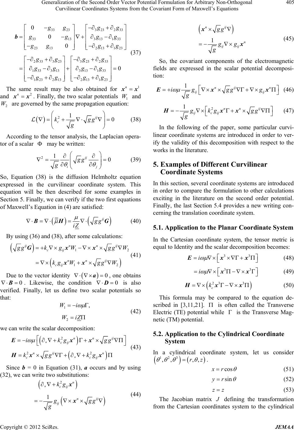

Generalization of the Second Order Vector Potential Formulation for Arbitrary Non-Orthogonal

Curvilinear Coordinates Systems from the Covariant Form of Maxwell’s Equations

405

33233 23233

33133 131 33

23132 131 23

233 323323 233

1 333 133 13133

1 232 132131 23

0

g

gg

ggg

g

gg

gg gg















 





 



 



b

g















(37)

The same result may be also obtained for 1n



xx

W

and . Finally, the two scalar potentials 1 and

are governed by the same propagation equation:

2nxx

2

W



210

ij

c

kgg

g









 (38)

According to the tensor analysis, the Laplacian opera-

tor of a scalar may be written:



210

ij

gg

g







 







(39)

So, Equation (38) is the diffusion Helmholtz equation

expressed in the curvilinear coordinate system. This

equation will be then described for some examples in

Section 5. Finally, we can verify if the two first equations

of Maxwell’s Equation in (4) are satisfied:





ij

gg

iZ



 



B

HG (40)

By using (36) and (38), after some calculations:



1

12

ijnn ij

cij

nn ij

cij

2

g

gkgW gg

kgWgg W

 



Gxx

xx

W

(41)

Due to the vector identity



0



 a, one obtains

0 

B

. Likewise, the condition 0

D

is also

verified. Finally, let us define two scalar potentials so

that:

1

2

,

Wi

WiZ





 



(42)

we can write the scalar decomposition:



2

22

n

nn ij

cij

nij n

ccij

ikg gg

kgg kg





 



 

Exx

Hx x



(43)

Since b = 0 in Equation (31), a occurs and by using

(32), we can write two substitutions:



2

1

n

cij

nij

ij

kg

gg

g





x





1

nij

n

ij ij

gg

g



 

x

(45)

So, the covariant components of the electromagnetic

fields are expressed in the scalar potential decomposi-

tion:

1nij n

ij ij

iggg g

g















Ex x

(46)

2

1nn ij

ijc ij

gkg gg

g







 





Hxx

(47)

In the following of the paper, some particular curvi-

linear coordinate systems are introduced in order to ver-

ify the validity of this decomposition with respect to the

works in the literature.

5. Examples of Different Curvilinear

Coordinate Systems

In this section, several coordinate systems are introduced

in order to compare the formulation to other calculations

exciting in the literature on the second order potential.

Finally, the last Section 5.4 provides a new writing con-

cerning the translation coordinate system.

5.1. Application to the Planar Coordinate System

In the Cartesian coordinate system, the tensor metric is

equal to Identity and the scalar decomposition becomes:

33

i









 





Exx

(48)

3

i



3







 





xx (49)





23 3

c

k



 Hxx (50)

This formula may be compared to the equation de-

scribed in [3,11,21].



is often called the Transverse

Electric (TE) potential while is the Transverse Mag-

netic (TM) potential.



5.2. Application to the Cylindrical Coordinate

System

In a cylindrical coordinate system, let us consider









123

,, ,,rz

 

.

cosxr





(51)

sinyr





(52)

zz



(53)

g

(44) The Jacobian matrix

J

defining the transformation

from the Cartesian coordinates system to the cylindrical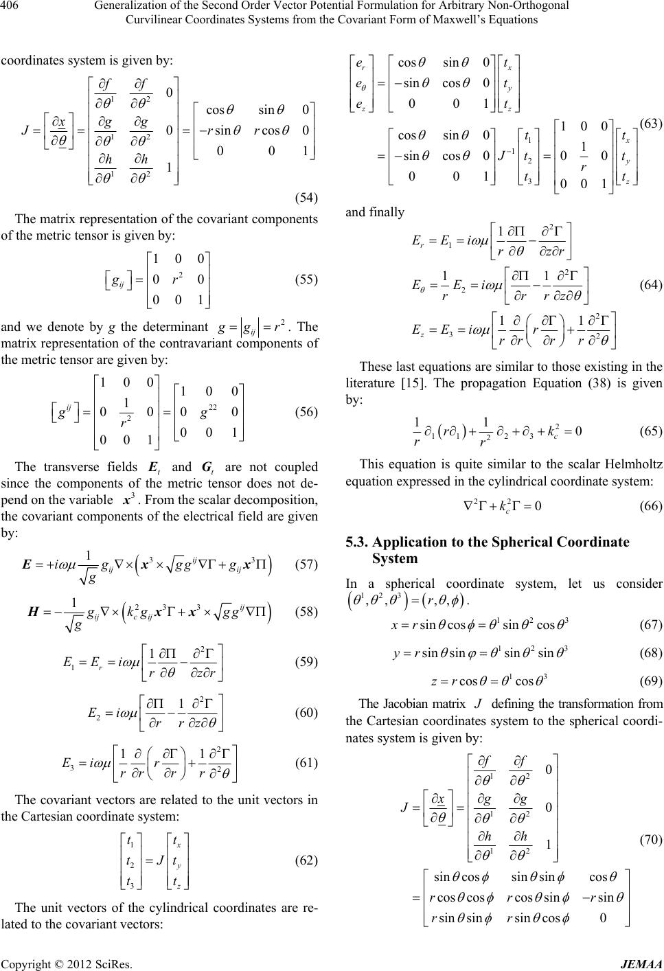

Generalization of the Second Order Vector Potential Formulation for Arbitrary Non-Orthogonal

Curvilinear Coordinates Systems from the Covariant Form of Maxwell’s Equations

406

coordinates system is given by:

12

0

cossin 0

0sincos

00

1

ff

xgg

Jr0

1

hh

 













 





 



 

 





 













0



r

(54)

The matrix representation of the covariant components

of the metric tensor is given by:

2

100

0

001

ij

gr















(55)

and we denote by g the determinant 2

ij

g

gr. The

matrix representation of the contravariant components of

the metric tensor are given by:

22

2

100100

1

000

001

ij

gg

r



0





































(56)

The transverse fields t

E

and t are not coupled

since the components of the metric tensor does not de-

pend on the variable . From the scalar decomposition,

the covariant components of the electrical field are given

by:

G

3

x



33

1ij

ij ij

ig ggg

g



Ex



x (57)



233

1ij

ijc ij

gkg gg

g

 Hxx (58)

2

1

r

EEi rz

 













r



(59)

2

1

Ei rrz







 













(60)

2

32

11

Eir

rrr r







 









 





(61)

The covariant vectors are related to the unit vectors in

the Cartesian coordinate system:

1

2

3

x

y

z

tt

tJt

tt

































(62)

The unit vectors of the cylindrical coordinates are re-

lated to the covariant vectors:

1

2

3

cossin 0

sincos 0

001

100

cossin 01

sincos 000

001001

rx

y

zz

x

y

z

et

tt

J

tt

r

tt







 

 



 

 









 







 

 







 













 



(63)

and finally

2

1

2

32

1

11

r

z

EEi rzr

EEi

rrrz

EEi r

rrr r



 









 









 

 











 



 







 







(64)

These last equations are similar to those existing in the

literature [15]. The propagation Equation (38) is given

by:



2

11 23

2

11 0

c

r

rrk



  (65)

This equation is quite similar to the scalar Helmholtz

equation expressed in the cylindrical coordinate system:

22

0

c

k



 (66)

5.3. Application to the Spherical Coordinate

System

In a spherical coordinate system, let us consider









123

,, ,,r



 



.

12

sin cossincosxr 3



 

 (67)

12

sin sinsinsinyr 3



 

 (68)

1

cos coszr 3





 (69)

The Jacobian matrix

J

defining the transformation from

the Cartesian coordinates system to the spherical coordi-

nates system is given by:

12

0

1

sin cossin sincos

cos coscos sinsin

sin sinsin cos0

ff

xgg

J

hh

rr r

rr











































































(70)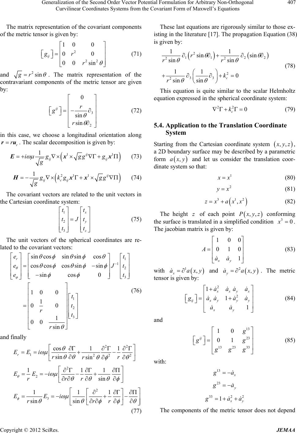

Generalization of the Second Order Vector Potential Formulation for Arbitrary Non-Orthogonal

Curvilinear Coordinates Systems from the Covariant Form of Maxwell’s Equations

407

The matrix representation of the covariant components

of the metric tensor is given by:

2

22

100

00

00 sin

ij

gr

r

















(71)

and 2singr



. The matrix representation of the

contravariant components of the metric tensor are given

by:

3

2

0

sin

ij r

g

r











 











(72)

in this case, we choose a longitudinal orientation along

. The scalar decomposition is given by:

r

rru



1

1ij

ij ij

ig ggg

g



Ex

1

x (73)



21 1

1ij

ijcij

gkggg

g

 Hxx

(74)

The covariant vectors are related to the unit vectors in

the Cartesian coordinate system:

1

2

3

x

y

z

tt

tJt

tt

 

 



 



(75)

The unit vectors of the spherical coordinates are re-

lated to the covariant vectors:

1

2

3

1

2

3

sin cossinsincos

cos coscos sinsin

sin cos0

10 0

1

00

1

00 sin

r

et

eJt

et

t

rt

r





 

 

































































(76)

and finally

22

1222

2

3

cos1 1

sin sin

111

sin

111

sin sin

r

EEi rr

r

EEi

rrr

EEi

rrr







   

 











 









 





 







 



 





These last equations are rigorously similar to those ex-

isting in the literature [17]. The propagation Equation (38)

is given by:



2

11 2

22

2

33

2

11

sin sin

11 0

sin

sin c

r

rr

k

r





2



 









(78)

This equation is quite similar to the scalar Helmholtz

equation expressed in the spherical coordinate system:

22

0

c

k



 (79)

5.4. Application to the Translation Coordinate

System

Starting from the Cartesian coordinate system





,,

x

yz ,

a 2D boundary surface may be described by a parametric

form





,axy and let us consider the translation coor-

dinate system so that:

1

x



(80)

2

y

x



(81)



31

,zx axx



2



(82)

The height of each point conforming

the surface is translated in a simplified condition

z



,,Pxyz

30x



.

The jacobian matrix is given by:

100

010

1

xy

A

aa

























(83)

with





1,

x

aax

y



y and . The metric

tensor is given by:



2,

y

aax



2

1

x

xy x

ijxyyy

xy

aaaa

g

aaaa

aa

































(84)

and

13

23

13 23 33

10

01

ij

g

gg



























(85)

with:

13

x

g

a







(77)

23

y

g

a





332 2

1

x

y

g

aa







The components of the metric tensor does not depend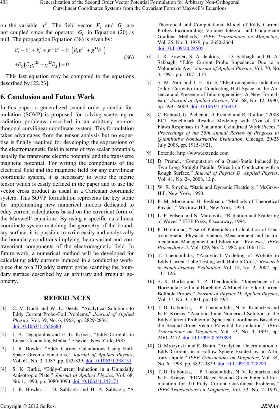

Generalization of the Second Order Vector Potential Formulation for Arbitrary Non-Orthogonal

Curvilinear Coordinates Systems from the Covariant Form of Maxwell’s Equations

408

on the variable . The field vector t

3

x

E

and t

G are

not coupled since the operator t in Equation (20) is

null. The propagation Equation (38) is given by:

G







22233 21313

12331 1

23 23

322 0

c

kgg g

gg

 

 

(86)

This last equation may be compared to the equations

described by [22,23].

6. Conclusion and Future Work

In this paper, a generalized second order potential for-

mulation (SOVP) is proposed for solving scattering or

radiation problems described in an arbitrary non-or-

thogonal curvilinear coordinate system. This formulation

takes advantages from the tensor analysis but no exper-

tise is finally required for developing the expressions of

the electromagnetic field in terms of two scalar potentials,

usually the transverse electric potential and the transverse

magnetic potential. For writing the components of the

electrical field and the magnetic field for any curvilinear

coordinate system, it is necessary to write the metric

tensor which is easily defined in the paper and to use the

vector cross product as usual in a Cartesian coordinate

system. This SOVP formulation represents the key stone

for implementing new numerical models dedicated to

eddy current calculations based on the covariant form of

the Maxwell’ equations. By using a specific curvilinear

coordinate system matching the geometry of the bound-

ary surface, it is possible to write easily and analytically

the boundary conditions implying the covariant and con-

travariant components of the electromagnetic field. In

future work, a numerical method will be developed for

calculating eddy currents induced in a conducting work-

piece due to a 3D eddy current probe scanning the boun-

dary surface described by an arbitrary and irregular ge-

ometry.

REFERENCES

[1] C. V. Dodd and W. E. Deeds, “Analytical Solutions to

Eddy Current Probe-Coil Problems,” Journal of Applied

Physics, Vol. 39, No. 6, 1968, pp. 2829-2838.

doi:10.1063/1.1656680

[2] J. A. Tegopoulos and E. E. Kriezis, “Eddy Currents in

Linear Conducting Media,” Elsevier, New York, 1985.

[3] J. R. Bowler, “Eddy Current Calculations Using Half-

Space Green’s Functions,” Journal of Applied Physics,

Vol. 61, No. 3, 1987, pp. 833-839. doi:10.1063/1.338131

[4] S. K. Burke, “Eddy-Current Induction in a Uniaxially

Anisotropic Plate,” Journal of Applied Physics, Vol. 68,

No. 1, 1990, pp. 3080-3090. doi:10.1063/1.347171

[5] J. R. Bowler, L. D. Sabbagh and H. A. Sabbagh, “A

Theoretical and Computational Model of Eddy Current

Probes Incorporating Volume Integral and Conjuguate

Gradient Methods,” IEEE Transactions on Magnetics,

Vol. 25, No. 3, 1989, pp. 2650-2664.

doi:10.1109/20.24505

[6] J. R. Bowler, S. A. Jenkins, L. D. Sabbagh and H. A.

Sabbagh, “Eddy Current Probe Impedance Due to a

Volumetric Aw,” Journal of Applied Physics, Vol. 70, No.

3, 1991, pp. 1107-1114.

[7] S. M. Nair and J. H. Rose, “Electromagnetic Induction

(Eddy Currents) in a Conducting Half-Space in the Ab-

sence and Presence of Inhomogeneities: A New Formal-

ism,” Journal of Applied Physics, Vol. 68, No. 12, 1990,

pp. 5995-6009. doi:10.1063/1.346933

[8] C. Reboud, G. Pichenot, D. Premel and R. Raillon, “2008

ECT Benchmark Results: Modeling with Civa of 3D

Flaws Responses in Planar and Cylindrical Work Pieces,”

Proceedings of the 35th Annual Review of Progress in

Quantitative Nondestructive Evaluation, Chicago, 20-25

July 2008, pp. 1915-1921.

[9] Extende. http://www.extende.com

[10] D. Prémel, “Computation of a Quasi-Static Induced by

Two Long Straight Parallel Wires in a Conductor with a

Rough Surface,” Journal of Physics D: Applied Physics,

Vol. 41, No. 24, 2008, 12 p.

[11] W. R. Smythe, “Static and Dynamic Electricity,” McGraw-

Hill, New York, 1950.

[12] P. M. Morse and H. Feshbach, “Methods of Theoretical

Physics,” McGraw-Hill, New York, 1953.

[13] L. P. Felsen and N. Marcuvitz, “Radiation and Scattering

of Waves,” IEEE Press, Piscataway, 1994.

[14] P. Hammond, “Use of Potentials in Calculation of Elec-

tromagnetic. Physical Science, Measurement and Instru-

mentation, Management and Education—Reviews,” IEEE

Proceedings A, Vol. 129, No. 2, 1982, pp. 106-112.

[15] T. Theodoulidis, “Analytical Modeling of Wobble in

Eddy Current Tube Testing with Bobbin Coils,” Research

in Nondestructive Evaluation, Vol. 14, No. 2, 2002, pp.

111-126.

[16] S. K. Burke and T. P. Theodoulidis, “Impedance of a

Horizontal Coil in a Borehole: A Model for Eddy-Current

Bolthole Probes,” Journal of Physics D: Applied Physics,

Vol. 37, No. 3, 2004, pp. 485-494.

[17] T. D. Tsiboukis, T. P. Theodoulidis, N. V. Kantartzis and

E. E. Kriezis, “Analytical and Numerical Solution of the

Eddy-Current Problem in Spherical Coordinates Based on

the Second-Order Vector Potential Formulation,” IEEE

Transactions on Magnetics, Vol. 33, No. 4, 1997, pp.

2461-2472. doi:10.1109/20.595899

[18] G. Mrozynski and E. Baum, “Analytical Determination of

Eddy Currents in a Hollow Sphere Excited by an Arbi-

trary Dipole,” IEEE Transactions on Magnetics, Vol. 34,

No. 6, 1998, pp. 3822-3829. doi:10.1109/20.728290

[19] T. D. Tsiboukis, T. P. Theodoulidis, N. V. Kantartzis and

E. E. Kriezis, “FDM-Based Second Order Potential For-

mulation for 3D Eddy Current Curvilinear Problems,”

IEEE Transactions on Magnetics, Vol. 33, No. 2, 1997,

Generalization of the Second Order Vector Potential Formulation for Arbitrary Non-Orthogonal

Curvilinear Coordinates Systems from the Covariant Form of Maxwell’s Equations

409

pp. 1287-1290. doi:10.1109/20.582490

[20] E. J. Post, “Formal Structure of Electromagnetics: Gen-

eral Covariance and Electromagnetics. (Series in Phys-

ics),” North Holland Publishing Company, Amsterdam,

1962.

[21] L. B. Felsen and N. Marcuvitz, “Radiation and Scattering

of Waves,” Prentice-Hall, Upper Saddle River, 1972.

[22] G. Granet, “Analysis of Diffraction by Surface-Relief

Crossed Gratings with Use of the Chan-Dezon Method:

Application to Multilayer Crossed Gratings,” Journal of

the Optical Society of American A, Vol. 15, No. 5, 1998,

pp. 1121-1131. doi:10.1364/JOSAA.15.001121

[23] K. A. Braham, R. Dusseaux and G. Granet, “Scattering of

Electromagnetic Waves from Two-Dimensional Perfectly

Conducting Random Rough Surfaces—Study with the

Curvilinear Coordinate Method,” Waves in Random Me-

dia, Vol. 18, No. 2, 2008, pp. 255-274.

doi:10.1080/17455030701749328

Paper Menu >>

Journal Menu >>