Accessing the Potential of Satellite and Telemetric Data to Evaluate the Influence of the Heat Flux Exchange in the Water Column Mixing and Stratification

doi:10.4236/ijg.2012.325092

Paper Menu >>

Journal Menu >>

International Journal of Geosciences, 2012, 3, 899-907

http://dx.doi.org/10.4236/ijg.2012.325092 Published Online October 2012 (http://www.SciRP.org/journal/ijg)

Accessing the Potential of Satellite and Telemetric Data to

Evaluate the Influence of the Heat Flux Exchange in the

Water Column Mixing and Stratification

Enner Alcântara

Department of Cartography, Sao Paulo State University (UNESP), Presidente Prudente, Brazil

Email: [email protected]

Received August 3, 2012; revised September 1, 2012; accepted October 2, 2012

ABSTRACT

The objective of this work is to evaluate the feasibility of moderate resolution satellite data estimating the surface heat

balance in a tropical hydroelectric reservoir. Each component of the heat flux balance was computed using the MODIS

(Moderate Resolution Imaging Spectroradiometer) water surface temperature (WST) level 2, 1 km nominal resolution

data (MOD11L2, version 5) from 2003 to 2008. The consequence of the heat flux exchange in the water column ther-

mal structure is also investigated. The passage of cold front over a region decreases the atmospheric pressure and air

temperature, enhancing the relative h umidity. The sensible flux presents a small variability b ut an increase occurs due to

a convective turbulence caused by front passage. The latent flux decrease but insufficiently to cause a co nd en sation, just

the evaporation decreases. The upwelling events are the responsible to maintain the loss o f heat after the cold front pas-

sage.

Keywords: Thermal Infrared; Heat and Cooling; Mixing; Stratification

1. Introduction

Aquatic systems continually respond to climatic con-

ditions (hydro-metrological processes) that vary over

broad scales of space and time. The primary control of

the seasonal cycle of water temperature at a given

location is the seasonal cycle of incoming shortwave

radiation. The response of each water body to meteo-

rological conditions is revealed firstly by the thermal

structure of the water column [1]. The precise knowl-

edge of reservoir heat flux dynamics is of paramount

relevance for hydrobiological and water quality studies

as physical control of the biotic structure in reservoirs is

even more important than in natu ral lakes [2].

Thermal infrared remote sensing applied to freshwater

ecosystems has aimed to map surface temperatures [3-5],

bulk temperatures [6], circulation patterns [7] and to

characterize upwelling events [8]. However, the appli-

cation of thermal infrared images to estimate the net heat

flux in tropical hydroelectric reservoirs is scarce.

Besides the power of thermal remote sensing images

to study the water surface temperature, the satellite data

is only from the upper most layer of the water surface

(skin temperature). To see below the surface some au-

thors had used telemetric data collected by an anchored

buoy [9,10].

Based on this, the objective of this paper is to estimate

the influence of the heat flux exchange between the wa-

ter surface and the atmosphere in the water column

stratification.

2. Methodology

2.1. Study Area

Our study site is the Itumbiara hydroelectric reservoir

(18˚25'S, 49˚06'W), located in a region stretched between

Minas Gerais and Goiás States (Central Brazil) that was

originally covered by tropical grassland savanna, cover-

ing an area of approximately 814 km2 and a volume of

17.03 billion m3 (Figure 1).

The climate in the region is characterized by an aver-

age precipitation ranging from 2.0 mm in the dry season

(May-September) to 315 mm in the rainy season (Oc-

tober-April). In the rainy season the wind intensity ran-

ges from 1.6 to 2.0 m·s–1 and reaches up to 3.0 m·s–1 in

the dry season, with the preferential wind direction from

the southeast. The air temperature in the rainy season

ranges from 25˚C to 26.5˚C dropping to 21˚C in June as

the dry season starts. The relative humidity has a pattern

similar to tha t of th e air temp erature, bu t with a s mall shift

in the minimum value towards September (47%). More-

ver, during the rainy season the humidity can reach 80%. o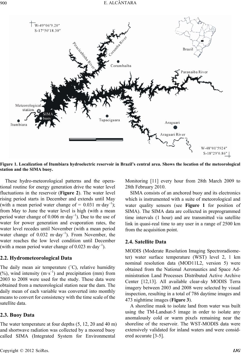

E. ALCÂNTARA

900

Figure 1. Localization of Itumbiara hydroelectric reservoir in Brazil’s central area. Shows the location of the meteorological

station and the SIMA buoy.

These hydro-meteorological patterns and the opera-

tional routine for energy generation drive the water level

fluctuations in the reservoir (Figure 2). The water level

rising period starts in December and extends until May

(with a mean period water change of = 0.031 m·day–1);

from May to June the water level is high (with a mean

period water change of 0.006 m·day–1). Due to the use of

water for power generation and evaporation rates, the

water level recedes until November (with a mean period

water change of 0.032 m·day–1). From November, the

water reaches the low level condition until December

(with a mean period water chang e of 0.023 m·day–1).

2.2. Hydrometeorological Data

The daily mean air temperature (˚C), relative humidity

(%), wind intensity (m·s–1) and precipitation (mm) from

2003 to 2008 were used for the study. These data were

obtained from a meteorological station near the dam. The

daily mean of each variable was converted into monthly

means to convert for consistency with the time scale of the

satellite data.

2.3. Buoy Data

The water temperatu re at four depths (5, 12, 20 and 40 m)

and shortwave radiation was collected by a moored buoy

called SIMA (Integrated System for Environmental

Monitoring [11] every hour from 28th March 2009 to

28th February 2010.

SIMA consis ts of an anchored buo y and its electron ics

which is instrumented with a suite of meteorological and

water quality sensors (see Figure 1 for position of

SIMA). The SIMA data are collected in preprogrammed

time intervals (1 hour) and are transmitted via satellite

link in quasi-real time to any user in a range of 2500 km

from the acquisition point.

2.4. Satellite Data

MODIS (Moderate Resolution Imaging Spectroradiome-

ter) water surface temperature (WST) level 2, 1 km

nominal resolution data (MOD11L2, version 5) were

obtained from the National Aeronautics and Space Ad-

ministration Land Processes Distributed Active Archive

Center [12,13]. All available clear-sky MODIS Terra

imagery between 2003 and 2008 were selected by visual

inspection, resulting in a total of 786 daytime images and

473 nighttime images (Figure 3).

A shoreline mask to isolate land from water was built

using the TM-Landsat-5 image in order to isolate any

anomalously cold or warm pixels remaining near the

shoreline of the reservoir. The WST-MODIS data were

extensively validated for inland waters and were consid-

ered accurate [3-5].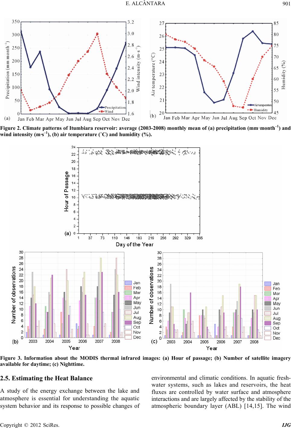

E. ALCÂNTARA 901

Figure 2. Climate patterns of Itumbiara reservoir: average (2003-2008) monthly mean of (a) precipitation (mm·month–1) and

wind intensity (m ·s–1), (b) air temperature (˚C) and humidity (%).

Figure 3. Information about the MODIS thermal infrared images: (a) Hour of passage; (b) Number of satellite imagery

available for daytime; (c) Nighttime.

2.5. Estimating the Heat Balance

A study of the energy exchange between the lake and

atmosphere is essential for understanding the aquatic

system behavior and its response to possible changes of

environmental and climatic conditions. In aquatic fresh-

water systems, such as lakes and reservoirs, the heat

fluxes are controlled by water surface and atmosphere

interactions and are largely affected by the stability of the

atmospheric boundary layer (ABL) [14,15]. The wind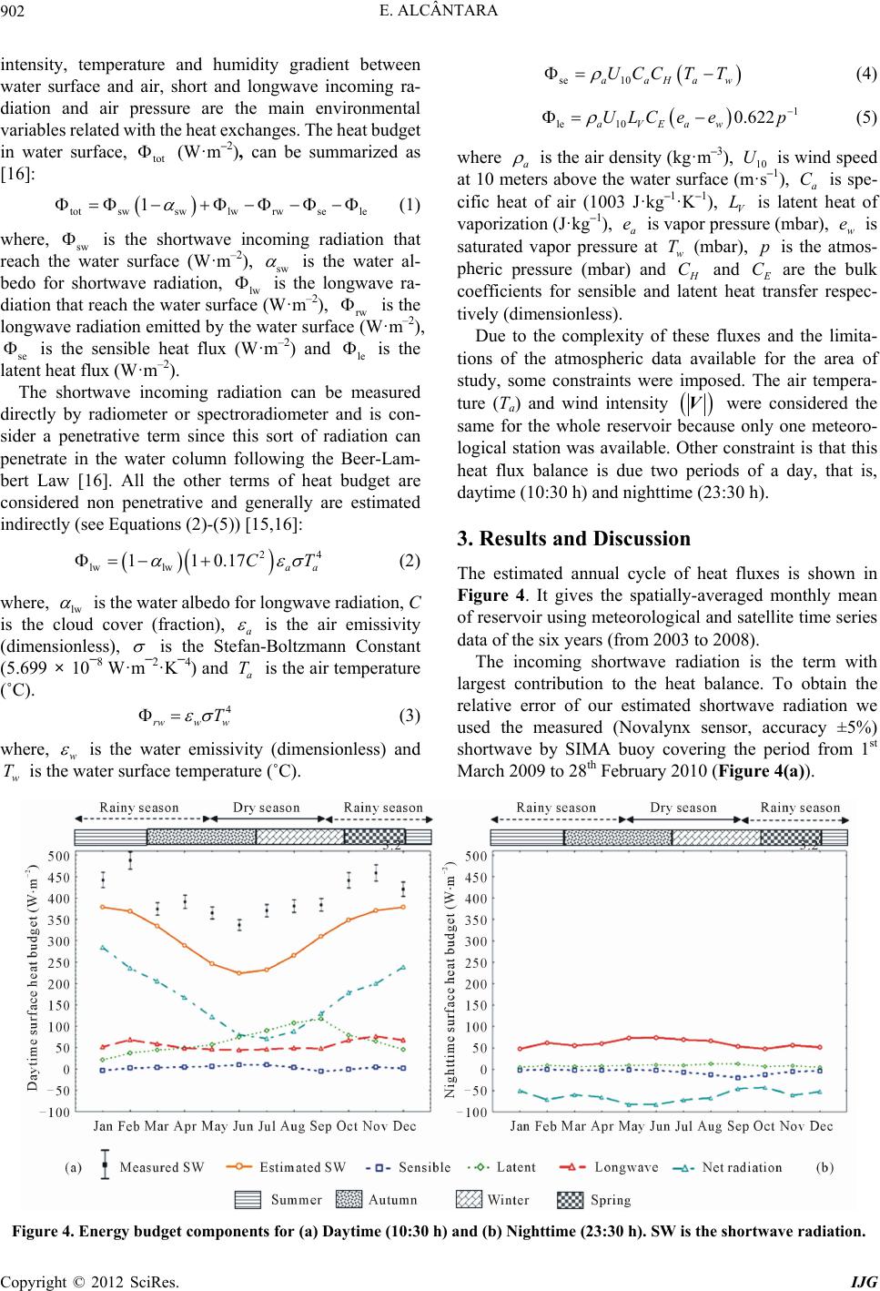

E. ALCÂNTARA

902

intensity, temperature and humidity gradient between

water surface and air, short and longwave incoming ra-

diation and air pressure are the main environmental

variables related wit h the he at exchange s. The heat budget

in water surface, (W·m–2), can be summarized as

[16]: tot



w se le







totswswlw r



  (1)

where, sw is the shortwave incoming radiation that

reach the water surface (W·m–2), sw



is the water al-

bedo for shortwave radiation, lw is the longwave ra-

diation that reach the water surface (W·m–2), rw is the

longwave radiation emitted by the water surface (W·m–2),

se is the sensible heat flux (W·m–2) and is the

latent heat flux (W·m–2).



le





017

The shortwave incoming radiation can be measured

directly by radiometer or spectroradiometer and is con-

sider a penetrative term since this sort of radiation can

penetrate in the water column following the Beer-Lam-

bert Law [16]. All the other terms of heat budget are

considered non penetrative and generally are estimated

indirectly (see Equations (2)-(5)) [15,16]:





lw lw





  (2)

where, lw



is the water al bed o f or lo ngwa ve radi ation, C

is the cloud cover (fraction), a



is the air emissivity

(dimensionless),



is the Stefan-Boltzmann Constant

(5.699 × 10–8 W·m–2·K–4) and is the air temperature

(˚C). a

rwww





 (3)

where, w



is the water emissivity (dimensionless) and

is the water surface temperature (˚C).





se 10aaHaw

UCC TT



 



(4)



le 100.622

aVEaw

ULCeep





 (5)

where a



is th e air density (kg·m–3), 10 is wind speed

at 10 meters above the water surface (m·s–1), a is spe-

cific heat of air (1003 J·kg–1·K–1), V is latent heat of

vaporization (J·kg–1), a is vapor pressu re (mbar), w is

saturated vapor pressure at (mbar), is the atmos-

pheric pressure (mbar) and

e e

T p

C and

C are the bulk

coefficients for sensible and latent heat transfer respec-

tively (dimensionless).

Due to the complexity of these fluxes and the limita-

tions of the atmospheric data available for the area of

study, some constraints were imposed. The air tempera-

ture (Ta) and wind intensity



V were considered the

same for the whole reservoir because only one meteoro-

logical station was available. Other constraint is that this

heat flux balance is due two periods of a day, that is,

daytime (10:30 h) and nigh ttime (23:30 h).

3. Results and Discussion

The estimated annual cycle of heat fluxes is shown in

Figure 4. It gives the spatially-averaged monthly mean

of reservoir using meteorological and satellite time series

data of the six years (from 2003 to 2008).

The incoming shortwave radiation is the term with

largest contribution to the heat balance. To obtain the

relative error of our estimated shortwave radiation we

used the measured (Novalynx sensor, accuracy ±5%)

shortwave by SIMA buoy covering the period from 1st

March 2009 to 28th February 2010 (Figure 4(a)).

Figure 4. Energy budget components for (a) Day t ime (10:30 h) and (b) Nighttime (23:30 h). SW is the shortwave radiation.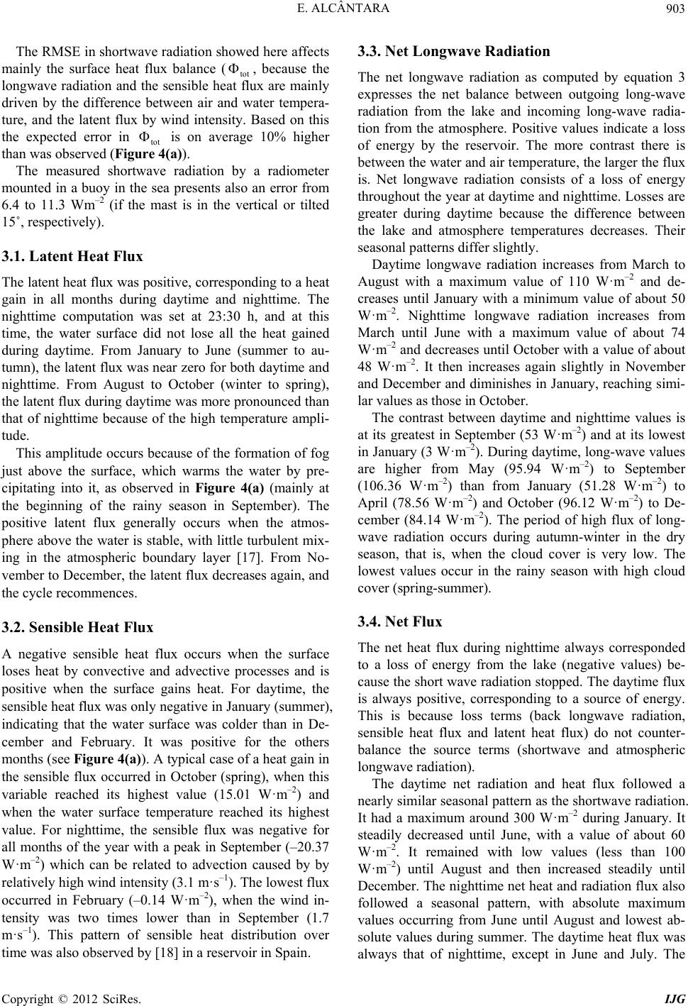

E. ALCÂNTARA 903

The RMSE in shortwave radiation showed here affects

mainly the surface heat flux balance (tot , because the

longwave radiation and the sensible heat flux are mainly

driven by the difference between air and water tempera-

ture, and the latent flux by wind intensity. Based on this

the expected error in tot is on average 10% higher

than was observed (Figu re 4 (a)).



The measured shortwave radiation by a radiometer

mounted in a buoy in the sea presents also an error from

6.4 to 11.3 Wm–2 (if the mast is in the vertical or tilted

15˚, respectively).

3.1. Latent Heat Flux

The latent heat flux was positive, correspond ing to a heat

gain in all months during daytime and nighttime. The

nighttime computation was set at 23:30 h, and at this

time, the water surface did not lose all the heat gained

during daytime. From January to June (summer to au-

tumn), the latent flux was near zero for both daytime and

nighttime. From August to October (winter to spring),

the latent flux during daytime was more pron ounced than

that of nighttime because of the high temperature ampli-

tude.

This amplitude occurs because of the formation of fog

just above the surface, which warms the water by pre-

cipitating into it, as observed in Figure 4(a) (mainly at

the beginning of the rainy season in September). The

positive latent flux generally occurs when the atmos-

phere above the water is stable, with little turbulent mix-

ing in the atmospheric boundary layer [17]. From No-

vember to December, the latent flux decreases again, and

the cycle recommences.

3.2. Sensible Heat Flux

A negative sensible heat flux occurs when the surface

loses heat by convective and advective processes and is

positive when the surface gains heat. For daytime, the

sensible heat flux was only negative in Janu ary (summer),

indicating that the water surface was colder than in De-

cember and February. It was positive for the others

months (see Figure 4(a)). A typical case of a heat gain in

the sensible flux occurred in October (spring), when this

variable reached its highest value (15.01 W·m–2) and

when the water surface temperature reached its highest

value. For nighttime, the sensible flux was negative for

all months of the year with a peak in September (–20.37

W·m–2) which can be related to advection caused by by

relatively high wind intensity (3.1 m·s–1). The lowest flux

occurred in February (–0.14 W·m–2), when the wind in-

tensity was two times lower than in September (1.7

m·s –1). This pattern of sensible heat distribution over

time was also observed by [18] in a reservoir in Spain.

3.3. Net Longwave Radiation

The net longwave radiation as computed by equation 3

expresses the net balance between outgoing long-wave

radiation from the lake and incoming long-wave radia-

tion from the atmosphere. Positive values indicate a loss

of energy by the reservoir. The more contrast there is

between the water and air temperature, the larger the flux

is. Net longwave radiation consists of a loss of energy

throughout th e year at daytime and nighttime. Losses are

greater during daytime because the difference between

the lake and atmosphere temperatures decreases. Their

seasonal patterns differ slightly.

Daytime longwave radiation increases from March to

August with a maximum value of 110 W·m–2 and de-

creases until January with a minimum value of about 50

W·m–2. Nighttime longwave radiation increases from

March until June with a maximum value of about 74

W·m–2 and decreases until October with a value of about

48 W·m–2. It then increases again slightly in November

and December and diminishes in January, reaching simi-

lar values as those in October.

The contrast between daytime and nighttime values is

at its greatest in September (53 W·m–2) and at its lowest

in January (3 W· m–2). During daytime, long-w ave values

are higher from May (95.94 W·m–2) to September

(106.36 W·m–2) than from January (51.28 W·m–2) to

April (78.56 W·m–2) and October (96.12 W·m–2) to De-

cember (84.14 W·m–2). The period of high flux of long-

wave radiation occurs during autumn-winter in the dry

season, that is, when the cloud cover is very low. The

lowest values occur in the rainy season with high cloud

cover (spri n g-summ e r).

3.4. Net Flux

The net heat flux during nighttime always corresponded

to a loss of energy from the lake (negative values) be-

cause the short wave radiation stopped. The daytime flux

is always positive, corresponding to a source of energy.

This is because loss terms (back longwave radiation,

sensible heat flux and latent heat flux) do not counter-

balance the source terms (shortwave and atmospheric

longwave radiation).

The daytime net radiation and heat flux followed a

nearly similar seasonal pattern as the shortwave radiation.

It had a maximum around 300 W·m–2 during January. It

steadily decreased until June, with a value of about 60

W·m–2. It remained with low values (less than 100

W·m–2) until August and then increased steadily until

December. The nighttime net heat and radiation flux also

followed a seasonal pattern, with absolute maximum

values occurring from June until August and lowest ab-

solute values during summer. The daytime heat flux was

always that of nighttime, except in June and July. The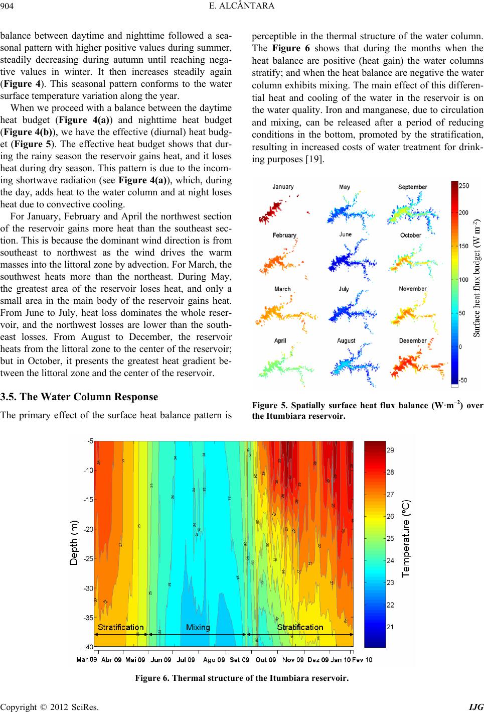

E. ALCÂNTARA

904

balance between daytime and nighttime followed a sea-

sonal pattern with high er positive values during summer,

steadily decreasing during autumn until reaching nega-

tive values in winter. It then increases steadily again

(Figure 4). This seasonal pattern conforms to the water

surface temperature variation along the year.

When we proceed with a balance between the daytime

heat budget (Figure 4(a)) and nighttime heat budget

(Figure 4(b)), we have the effective (diurnal) heat budg-

et (Figure 5). The effective heat budget shows that dur-

ing the rainy season the reservoir gains heat, and it loses

heat during dry season. This pattern is due to the incom-

ing shortwave radiation (see Figure 4(a)), which, during

the day, adds heat to the water column and at night loses

heat due to convective cooling.

For January, February and April the northwest section

of the reservoir gains more heat than the southeast sec-

tion. This is because the dominant wind direction is from

southeast to northwest as the wind drives the warm

masses into the littoral zo ne by adv ection . Fo r March, the

southwest heats more than the northeast. During May,

the greatest area of the reservoir loses heat, and only a

small area in the main body of the reservoir gains heat.

From June to July, heat loss dominates the whole reser-

voir, and the northwest losses are lower than the south-

east losses. From August to December, the reservoir

heats from the littoral zone to the center of the reservoir;

but in October, it presents the greatest heat gradient be-

tween the littoral zone and the center of the reservoir.

3.5. The Water Column Response

The primary effect of the surface heat balance pattern is

perceptible in the thermal structure of the water column.

The Figure 6 shows that during the months when the

heat balance are positive (heat gain) the water columns

stratify; and when the heat balance are negative the water

column exhibits mixing. The main effect of this differen-

tial heat and cooling of the water in the reservoir is on

the water quality. Iron and manganese, due to circulation

and mixing, can be released after a period of reducing

conditions in the bottom, promoted by the stratification,

resulting in increased costs of water treatment for drink-

ing purpo ses [19].

Figure 5. Spatially surface heat flux balance (W·m–2) over

the Itumbiara reservoir.

Figure 6. Thermal structure of the Itumbiara reservoir.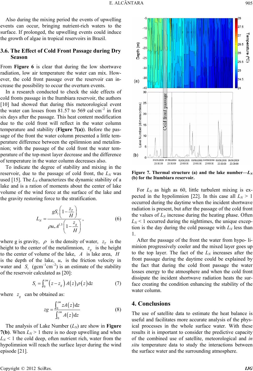

E. ALCÂNTARA 905

Also during the mixing period the events of upwelling

events can occur, bringing nutrient-rich waters to the

surface. If prolonged, the upwelling events could induce

the growth of algae in tropical reservoirs in Brazil.

3.6. The Effect of Cold Front Passage during Dry

Season

From Figure 6 is clear that during the low shortwave

radiation, low air temperature the water can mix. How-

ever, the cold front passage over the reservoir can in-

crease the possibility to o ccur the overturn events.

In a research conducted to check the side effects of

cold fronts passage in th e Itumbiara reservoir, the authors

[10] had showed that during this meteorological event

the water can losses from 81.57 to 569 cal·cm–2 in first

six days after the passage. This heat content modification

due to the cold front will reflect in the water column

temperature and stability (Figure 7(a)). Before the pas-

sage of the front the water column presented a little te m-

perature difference between the epilimnion and metalim-

nion; with the passage of the cold front the water tem-

perature of the top-most layer decrease and the difference

of temperature in the water column decreases also.

To indicate the degree of stability and mixing in the

reservoir, due to the passage of cold front, the LN was

used [15]. The LN characterizes the dynamic stability of a

lake and is a ration of moments about the center of lake

volume of the wind force at the surface of the lake and

the gravity restoring force to the stratification.

1.5

gS Hz





















, (6)

where g is grav ity,



is the density of water, T is the

height to the cen ter of the metalimnion, z

z is the height

to the center of volume of the lake,

is lake area,

is the depth of the lake, * is the friction velocity in

water and t (gcm–1cm–2) is an estimate of the stability

of the reservoir calculated as [20]:



Sz



 

dzAzzz



(7)

where



can be obtained as:

zA zz



 (8)

The analysis of Lake Number (LN) are sh ow in Figure

7(b). When LN > 1 there is no deep upwelling and when

LN < 1 the cold deep, often nutrient rich, water from the

hypolimnion will reach the surface layer during the wind

episode [21].

Figure 7. Thermal structure (a) and the lake number—LN

(b) for the Itumbiara reservoir.

For LN as high as 60, little turbulent mixing is ex-

pected in the hypolimnion [22]. In this case all LN > 1

occurred dur ing the dayti me when the in cident sh ortwave

radiation is present, but after the passage of the cold front

the values of LN increase during the heating phase. Often

LN < 1 occurred during the nighttimes, the unique excep-

tion is the day during the cold passage with LN less than

1. After the passage of the front the water from hypo- li-

minion progressively cooler and the mixed layer goes up

to the top layer. The fact of the LN increases after the

front passage during the daytime could be explained by

the fact that during the cold front passage the water

losses energy to the atmosphere and when the cold front

dissipate the incident shortwave radiation heats the sur-

face creating the condition enhancing the stability of the

water column.

4. Conclusions

The use of satellite data to estimate the heat balance is

useful and facilitates more accurate analysis of the phys-

ical processes in the whole surface water. With these

results it is important to consider the predictive capacity

of the combined use of satellite, meteorological and in

situ temperature data to study the interactions between

the surface water and the surrounding atmosphere.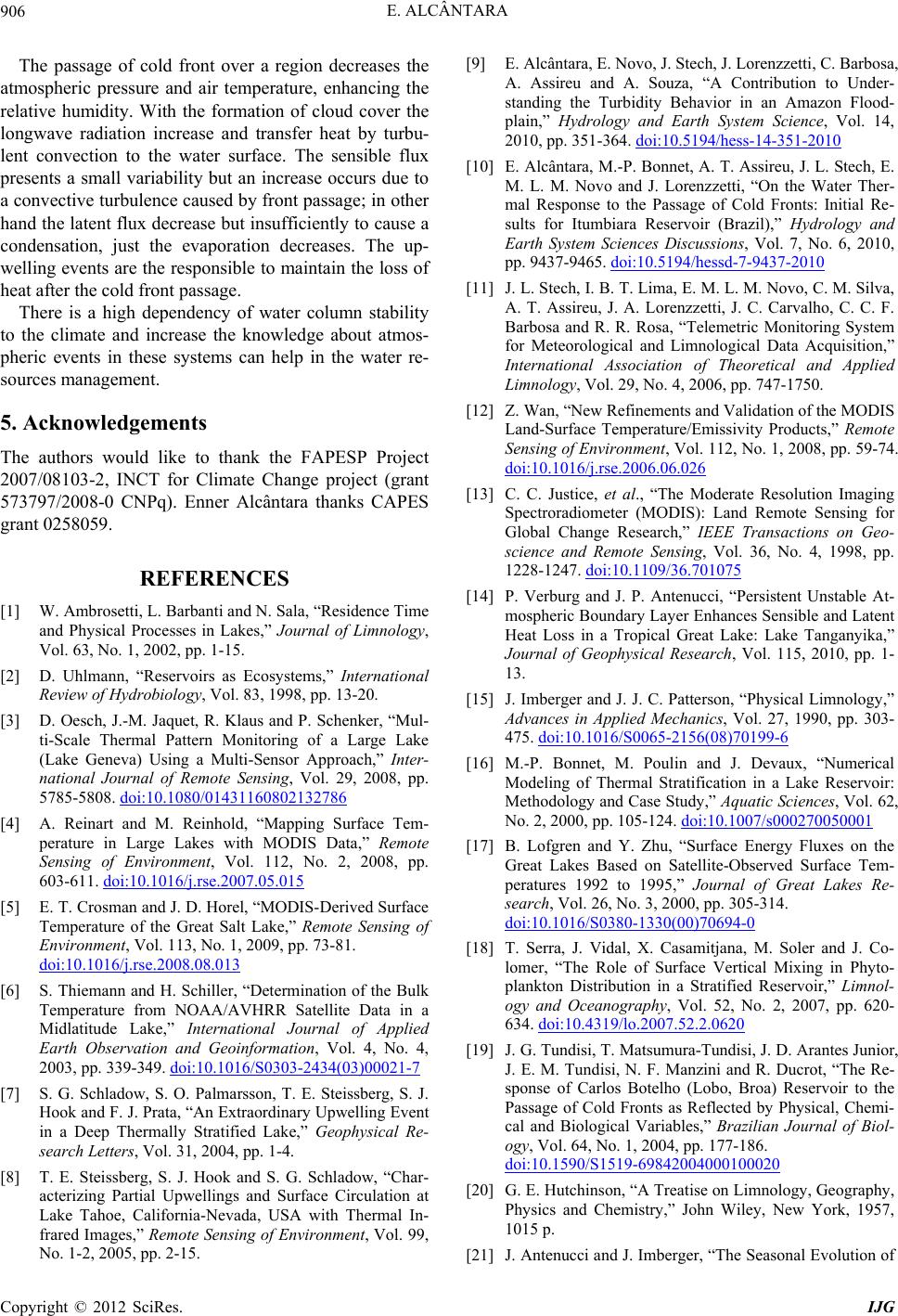

E. ALCÂNTARA

906

The passage of cold front over a region decreases the

atmospheric pressure and air temperature, enhancing the

relative humidity. With the formation of cloud cover the

longwave radiation increase and transfer heat by turbu-

lent convection to the water surface. The sensible flux

presents a small variability but an increase occurs due to

a convective turbulence caused by front passage; in other

hand the latent flux decrease but insufficiently to cause a

condensation, just the evaporation decreases. The up-

welling events are the responsible to maintain the loss of

heat after the cold front passage.

There is a high dependency of water column stability

to the climate and increase the knowledge about atmos-

pheric events in these systems can help in the water re-

sources management.

5. Acknowledgements

The authors would like to thank the FAPESP Project

2007/08103-2, INCT for Climate Change project (grant

573797/2008-0 CNPq). Enner Alcântara thanks CAPES

grant 0258059.

REFERENCES

[1] W. Ambrosetti, L. Barbanti and N. Sala, “Residence Time

and Physical Processes in Lakes,” Journal of Limnology,

Vol. 63, No. 1, 2002, pp. 1-15.

[2] D. Uhlmann, “Reservoirs as Ecosystems,” International

Review of Hydrobiology, Vol. 83, 1998, pp. 13-20.

[3] D. Oesch, J.-M. Jaquet, R. Klaus and P. Schenker, “Mul-

ti-Scale Thermal Pattern Monitoring of a Large Lake

(Lake Geneva) Using a Multi-Sensor Approach,” Inter-

national Journal of Remote Sensing, Vol. 29, 2008, pp.

5785-5808. doi:10.1080/01431160802132786

[4] A. Reinart and M. Reinhold, “Mapping Surface Tem-

perature in Large Lakes with MODIS Data,” Remote

Sensing of Environment, Vol. 112, No. 2, 2008, pp.

603-611. doi:10.1016/j.rse.2007.05.015

[5] E. T. Crosman and J. D. Horel, “MODIS-Derived Surface

Temperature of the Great Salt Lake,” Remote Sensing of

Environment, Vol. 113, No. 1, 2009, pp. 73-81.

doi:10.1016/j.rse.2008.08.013

[6] S. Thiemann and H. Schiller, “Determination of the Bulk

Temperature from NOAA/AVHRR Satellite Data in a

Midlatitude Lake,” International Journal of Applied

Earth Observation and Geoinformation, Vol. 4, No. 4,

2003, pp. 339-349. doi:10.1016/S0303-2434(03)00021-7

[7] S. G. Schladow, S. O. Palmarsson, T. E. Steissberg, S. J.

Hook and F. J. Prata, “An Extraordinary Upwelling Event

in a Deep Thermally Stratified Lake,” Geophysical Re-

search Letters, Vol. 31, 2004, pp. 1-4.

[8] T. E. Steissberg, S. J. Hook and S. G. Schladow, “Char-

acterizing Partial Upwellings and Surface Circulation at

Lake Tahoe, California-Nevada, USA with Thermal In-

frared Images,” Remote Sensing of Environment, Vol. 99,

No. 1-2, 2005, pp. 2-15.

[9] E. Alcântara, E. Novo, J. Stech, J. Lorenzzetti, C. Barbosa,

A. Assireu and A. Souza, “A Contribution to Under-

standing the Turbidity Behavior in an Amazon Flood-

plain,” Hydrology and Earth System Science, Vol. 14,

2010, pp. 351-364. doi:10.5194/hess-14-351-2010

[10] E. Alcântara, M.-P. Bonnet, A. T. Assireu, J. L. Stech, E.

M. L. M. Novo and J. Lorenzzetti, “On the Water Ther-

mal Response to the Passage of Cold Fronts: Initial Re-

sults for Itumbiara Reservoir (Brazil),” Hydrology and

Earth System Sciences Discussions, Vol. 7, No. 6, 2010,

pp. 9437-9465. doi:10.5194/hessd-7-9437-2010

[11] J. L. Stech, I. B. T. Lima, E. M. L. M. Novo, C. M. Silva,

A. T. Assireu, J. A. Lorenzzetti, J. C. Carvalho, C. C. F.

Barbosa and R. R. Rosa, “Telemetric Monitoring System

for Meteorological and Limnological Data Acquisition,”

International Association of Theoretical and Applied

Limnology, Vol. 29, No. 4, 2006, pp. 747-1750.

[12] Z. Wan, “New Refi nements and Validation of the MODIS

Land-Surface Temperature/Emissivity Products,” Remote

Sensing of Environment, Vol. 112, No. 1, 2008, pp. 59-74.

doi:10.1016/j.rse.2006.06.026

[13] C. C. Justice, et al., “The Moderate Resolution Imaging

Spectroradiometer (MODIS): Land Remote Sensing for

Global Change Research,” IEEE Transactions on Geo-

science and Remote Sensing, Vol. 36, No. 4, 1998, pp.

1228-1247. doi:10.1109/36.701075

[14] P. Verburg and J. P. Antenucci, “Persistent Unstable At-

mospheric Boundary Layer Enhances Sensible and Latent

Heat Loss in a Tropical Great Lake: Lake Tanganyika,”

Journal of Geophysical Research, Vol. 115, 2010, pp. 1-

13.

[15] J. Imberger and J. J. C. Patterson, “Physical Limnology,”

Advances in Applied Mechanics, Vol. 27, 1990, pp. 303-

475. doi:10.1016/S0065-2156(08)70199-6

[16] M.-P. Bonnet, M. Poulin and J. Devaux, “Numerical

Modeling of Thermal Stratification in a Lake Reservoir:

Methodology and Case Study,” Aquatic Sciences, Vol. 62,

No. 2, 2000, pp. 105-124. doi:10.1007/s000270050001

[17] B. Lofgren and Y. Zhu, “Surface Energy Fluxes on the

Great Lakes Based on Satellite-Observed Surface Tem-

peratures 1992 to 1995,” Journal of Great Lakes Re-

search, Vol. 26, No. 3, 2000, pp. 305-314.

doi:10.1016/S0380-1330(00)70694-0

[18] T. Serra, J. Vidal, X. Casamitjana, M. Soler and J. Co-

lomer, “The Role of Surface Vertical Mixing in Phyto-

plankton Distribution in a Stratified Reservoir,” Limnol-

ogy and Oceanography, Vol. 52, No. 2, 2007, pp. 620-

634. doi:10.4319/lo.2007.52.2.0620

[19] J. G. Tundisi, T. Matsumura-Tundisi, J. D. Arantes Junior,

J. E. M. Tundisi, N. F. Manzini and R. Ducrot, “The Re-

sponse of Carlos Botelho (Lobo, Broa) Reservoir to the

Passage of Cold Fronts as Reflected by Physical, Chemi-

cal and Biological Variables,” Brazilian Journal of Biol-

ogy, Vol. 64, No. 1, 2004, pp. 177-186.

doi:10.1590/S1519-69842004000100020

[20] G. E. Hutchinson, “A Treatise on Limnology, Geography,

Physics and Chemistry,” John Wiley, New York, 1957,

1015 p.

[21] J. Antenucci and J. Imberger, “The Seasonal Evolution of

E. ALCÂNTARA

907

Wind/Internal Wave Resonance in Lake Kinneret,” Lim-

nology and Oceanography, Vol. 48, No. 5, 2003, pp.

2055-2061. doi:10.4319/lo.2003.48.5.2055

[22] M. Hondzo and H. G. Stefan, “Long-Term Water Quality

Predictors,” Water Research, Vol. 30, No. 12, 1996, pp.

2835-2852. doi:10.1016/0043-1354(95)00286-3