Theory of Conductivity in Semiconducting Single-Wall Carbon Nanotubes

doi:10.4236/jmp.2012.310191

Paper Menu >>

Journal Menu >>

Journal of Modern Physics, 2012, 3, 1550-1555

http://dx.doi.org/10.4236/jmp.2012.310191 Published Online October 2012 (http://www.SciRP.org/journal/jmp)

Theory of Conductivity in Semiconducting Single-Wall

Carbon Nanotubes

Shigeji Fujita1, Salvador Godoy2, Akira Suzuki3*

1Department of Physics, University at Buffalo, Buffalo, USA

2Departamento de Física, Facultad de Ciencias, Universidad Nacional Autónoma de México, Mexico City, Mexico

3Department of Physics, Faculty of Science, Tokyo University of Science, Shinjuku-ku, Japan

Email: *[email protected]

Received August 13, 2012; revised September 16, 2012; accepted September 23, 2012

ABSTRACT

The conduction of a single-wall carbon nanotube depends on the pitch. If there are an integral number of carbon hexa-

gons per pitch, then the system is periodic along the tube axis and allows “holes” (not “electrons”) to move inside the

tube. This case accounts for a semiconducting behavior with the activation energy of the order of around 3 meV. There

is a distribution of the activation energy since the pitch and the circumference can vary. Otherwise nanotubes show me-

tallic behaviors (significantly higher conductivity). “Electrons” and “holes” can move in the graphene wall (two dimen-

sions). The conduction in the wall is the same as in graphene if the finiteness of the circumference is disregarded. Coo-

per pairs formed by the phonon exchange attraction moving in the wall is shown to generate a temperature-independent

conduction at low temperature (3 - 20 K).

Keywords: Semiconducting SWNT; Cartesian Unit Cell Model; Cooper Pair; Bloch Electron Dynamics

1. Introduction

Iijima [1] found after his electron diffraction analysis

that carbon nanotubes ranging 4 to 30 nanometers (nm)

in diameter have helical multi-walled structures. Single-

wall nanotube (SWNT) has about one nanometer in di-

ameter and micrometers (μm) in length. Ebbesen et al. [2]

measured the electrical conductivity



of individual

carbon nanotubes and found that



varies depending of

the temperature T, the tube radius r and the pitch p. Ex-

periments show that SWNT can be either semiconducting

or metallic, depending on how they are rolled up from

the graphene sheets [3]. In the present work we shall

present a microscopic theory of the electrical conductiv-

ity of semiconducting SWNT, starting with a graphene

honeycomb lattice, developing a Bloch electron dynam-

ics based on a rectangular cell model [4], and using ki-

netic theory. A SWNT can be formed by rolling a gra-

phene sheet into a circular cylinder. The graphene which

forms a honeycomb lattice is intrinsically anisotropic as

we shall explain it in more detail later in Section 2. Mo-

riyama et al. [5] fabricated 12 SWNT devices from one

chip, and observed that two of the SWNT samples are

semiconducting and the other 10 are metallic. The semi-

conducting SWNT samples show an activated-state tem-

perature behavior. That is, the resistance decreases with

increasing temperature. Why are there two sets of sam-

ples showing very different behavior? The answer to this

question is as follows.

The line passing the centers of the nearest-neighbor

carbon hexagons forms a helical line around the nano-

tube with a pitch p and a radius r.

In Figure 1(a), a section of the circular tube with a

pitch p is drawn. Its unrolled plane is shown in (b). The

circumference likely contains an integral number

m of the carbon hexagons (units). The pitch p, however,

may or may not contain an integral number n of units. In

the fabrication process the pitch is not controlled. In the

first alternative, the nanotube is periodic with the period

p along the tube axis. Then, there is a one-dimensional

(1D) k-vector along the tube. A “hole” which has a posi-

tive charge +e and a size of a unit ring of height p and

radius r can go through inside the positively charged

carbon wall. An “electron” having a negative charge −e

and a similar size is attracted by the carbon wall, and

hence it cannot go straight inside the wall. Thus, there

should be an extra “hole” channel current in a SWNT.

Moriyama et al. [5] observed a “hole”-like current after

examining the gate voltage effect. The system should

have the lowest energy if the unit ring contains an integer

set

2πr





,mn of carbon hexagons, which may be attained

*Corresponding author.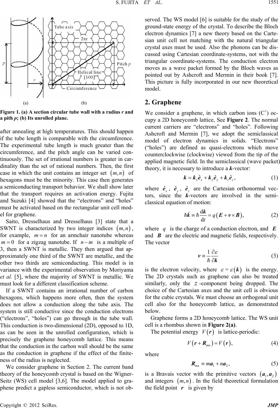

S. FUJITA ET AL. 1551

(a) (b)

Figure 1. (a) A section circular tube wall with a radius r and

a pith p; (b) Its unrolled plane.

after annealing at high temperatures. This should happen

if the tube length is comparable with the circumference.

The experimental tube length is much greater than the

circumference, and the pitch angle can be varied con-

tinuously. The set of irrational numbers is greater in car-

dinality than the set of rational numbers. Then, the first

case in which the unit contains an integer set





,mn of

hexagons must be the minority. This case then generates

a semiconducting transport behavior. We shall show later

that the transport requires an activation energy. Fujita

and Suzuki [4] showed that the “electrons” and “holes”

must be activated based on the rectangular unit cell mod-

el for graphene.

Saito, Dresselhaus and Dresselhaus [3] state that a

SWNT is characterized by two integer indices





,mn

mn

ˆˆˆ

for example, for an armchair nanotube whereas

for a zigzag nanotube. If is a multiple of

3, then a SWNT is metallic. They then argued that ap-

proximately one third of the SWNT are metallic, and the

other two thirds are semiconducting. This model is in

variance with the experimental observation by Moriyama

et al. [5], where the majority of SWNT is metallic. We

must look for a different classification scheme.

0mnm

If a SWNT contains an irrational number of carbon

hexagons, which happens more often, then the system

does not allow a conduction along the tube axis. The

system is still conductive since the conduction electrons

(“electrons”, “holes”) can go through in the tube wall.

This conduction is two-dimensional (2D), opposed to 1D,

as can be seen in the unrolled configuration, which is

precisely the graphene honeycomb lattice. This means

that the conduction in the carbon wall should be the same

as the conduction in graphene if the effect of the finite-

ness of the radius is neglected.

We consider graphene in Section 2. The current band

theory of the honeycomb crystal is based on the Wigner-

Seitz (WS) cell model [3,6]. The model applied to gra-

phene predict a gapless semiconductor, which is not ob-

served. The WS model [6] is suitable for the study of the

ground-state energy of the crystal. To describe the Bloch

electron dynamics [7] a new theory based on the Carte-

sian unit cell not matching with the natural triangular

crystal axes must be used. Also the phonons can be dis-

cussed using Cartesian coordinate-systems, not with the

triangular coordinate-systems. The conduction electron

moves as a wave packet formed by the Bloch waves as

pointed out by Ashcroft and Mermin in their book [7].

This picture is fully incorporated in our new theoretical

model.

2. Graphene

We consider a graphene, in which carbon ions (C+) oc-

cupy a 2D honeycomb lattice, See Figure 2. The normal

current carriers are “electrons” and “holes”. Following

Ashcroft and Mermin [7], we adopt the semiclassical

model of electron dynamics in solids. “Electrons”

(“holes”) are defined as quasi-electrons which move

counterclockwise (clockwise) viewed from the tip of the

applied magnetic field. In the semiclassical (wave packet)

theory, it is necessary to introduce a k-vector:

xyyzz



kke keke

(1)

where

eˆ

e are the Cartesian orthonormal vec-

tors, since the k-vectors are involved in the semi-

classical equation of motion:





kEvB





(2)

where is the charge of a conduction electron, and

and are the electric and magnetic fields, respectively.

The vector











(3)

is the electron velocity, where is the energy.

The 2D crystals such as graphene can also be treated

similarly, only the -component being dropped. The

choice of the Cartesian axes and the unit cell is obvious

for the cubic crystals. We must choose an orthogonal unit

cell also for the honeycomb lattice, as demonstrated

below.

Graphene forms a 2D honeycomb lattice. The WS unit

cell is a rhombus shown in Figure 2(a).





Vr is lattice-periodic: The potential energy







VVrR r

mn mn

(4)

where



Raa (5)



is a Bravais vector with the primitive vectors



,aa

and integers





,mn

r. In the field theoretical formulation

the field point is given by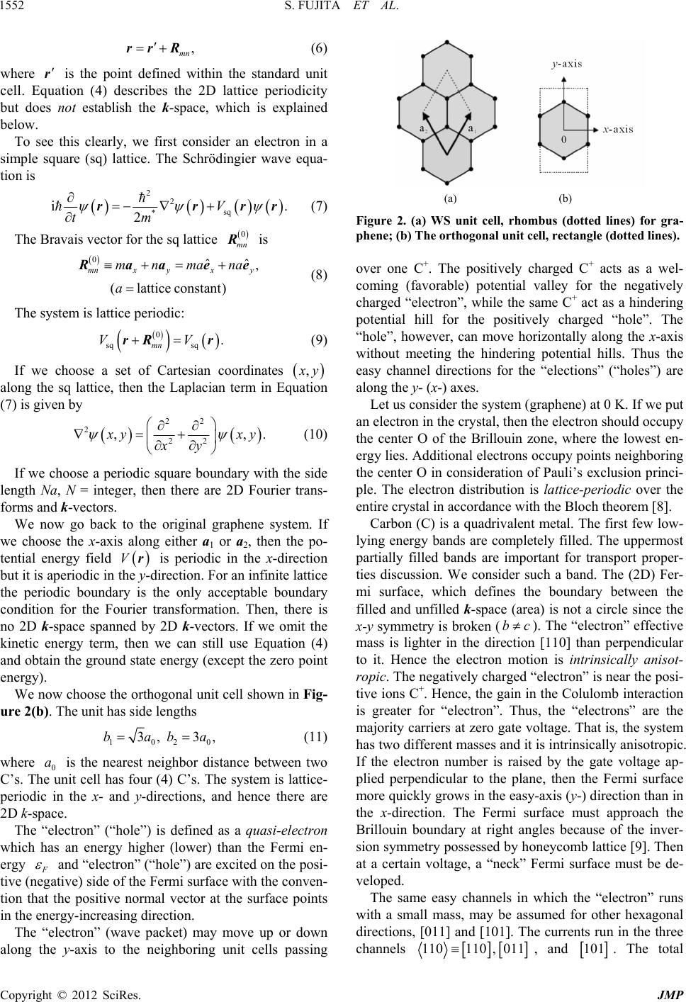

S. FUJITA ET AL.

1552





rrR



(6)

where is the point defined within the standard unit

cell. Equation (4) describes the 2D lattice periodicity

but does not establish the k-space, which is explained

below.

To see this clearly, we first consider an electron in a

simple square (sq) lattice. The Schrödingier wave equa-

tion is

 



 

rrrr





ˆˆ,

nstant)

x y

mana ee



mn Vr

. (7)

The Bravais vector for the sq lattice is



(lattice co

mnx y

a

Raamn (8)

The system is lattice periodic:

VrR . (9)

If we choose a set of Cartesian coordinates





along the sq lattice, then the Laplacian term in Equation

(7) is given by

 

22 ,.

yxy



















 (10)

If we choose a periodic square boundary with the side

length Na, N = integer, then there are 2D Fourier trans-

forms and k-vectors.

We now go back to the original graphene system. If

we choose the x-axis along either a1 or a2, then the po-

tential energy field is periodic in the x-direction

but it is aperiodic in the y-direction. For an infinite lattice

the periodic boundary is the only acceptable boundary

condition for the Fourier transformation. Then, there is

no 2D k-space spanned by 2D k-vectors. If we omit the

kinetic energy term, then we can still use Equation (4)

and obtain the ground state energy (except the zero point

energy).

We now choose the orthogonal unit cell shown in Fig-

ure 2(b). The unit has side lengths

1020

3, 3,baba

(11)

where 0 is the nearest neighbor distance between two

C’s. The unit cell has four (4) C’s. The system is lattice-

periodic in the x- and y-directions, and hence there are

2D k-space.

The “electron” (“hole”) is defined as a quasi-electron

which has an energy higher (lower) than the Fermi en-

ergy



and “electron” (“hole”) are excited on the posi-

tive (negative) side of the Fermi surface with the conven-

tion that the positive normal vector at the surface points

in the energy-increasing direction.

The “electron” (wave packet) may move up or down

along the y-axis to the neighboring unit cells passing

(a) (b)

Figure 2. (a) WS unit cell, rhombus (dotted lines) for gra-

phene; (b) The orthogonal unit cell, rectangle (dotted lines).

over one C+. The positively charged C+ acts as a wel-

coming (favorable) potential valley for the negatively

charged “electron”, while the same C+ act as a hindering

potential hill for the positively charged “hole”. The

“hole”, however, can move horizontally along the x-axis

without meeting the hindering potential hills. Thus the

easy channel directions for the “elections” (“holes”) are

along the y- (x-) axes.

Let us consider the system (graphene) at 0 K. If we put

an electron in the crystal, then the electron should occupy

the center O of the Brillouin zone, where the lowest en-

ergy lies. Additional electrons occupy points neighboring

the center O in consideration of Pauli’s exclusion princi-

ple. The electron distribution is lattice-periodic over the

entire crystal in accordance with the Bloch theorem [8].

Carbon (C) is a quadrivalent metal. The first few low-

lying energy bands are completely filled. The uppermost

partially filled bands are important for transport proper-

ties discussion. We consider such a band. The (2D) Fer-

mi surface, which defines the boundary between the

filled and unfilled k-space (area) is not a circle since the

x-y symmetry is broken (bc



). The “electron” effective

mass is lighter in the direction [110] than perpendicular

to it. Hence the electron motion is intrinsically anisot-

ropic. The negatively charged “electron” is near the posi-

tive ions C+. Hence, the gain in the Colulomb interaction

is greater for “electron”. Thus, the “electrons” are the

majority carriers at zero gate voltage. That is, the system

has two different masses and it is intrinsically anisotropic.

If the electron number is raised by the gate voltage ap-

plied perpendicular to the plane, then the Fermi surface

more quickly grows in the easy-axis (y-) direction than in

the x-direction. The Fermi surface must approach the

Brillouin boundary at right angles because of the inver-

sion symmetry possessed by honeycomb lattice [9]. Then

at a certain voltage, a “neck” Fermi surface must be de-

veloped.

The same easy channels in which the “electron” runs

with a small mass, may be assumed for other hexagonal

directions, [011] and [101]. The currents run in the three

channels









, and





101 . The total 110110 ,011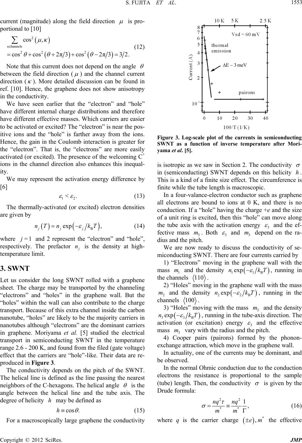

S. FUJITA ET AL. 1553

current (magnitude) along the field direction



is pro-

portional to [10]





channels

22 2

cos ,

cos cos2π3cos2π332.





 

 

 (12)

E3meV





Note that this current does not depend on the angle



between the field direction (



) and the channel current

direction (). More detailed discussion can be found in

ref. [10]. Hence, the graphene does not show anisotropy

in the conductivity.



We have seen earlier that the “electron” and “hole”

have different internal charge distributions and therefore

have different effective masses. Which carriers are easier

to be activated or excited? The “electron” is near the pos-

itive ions and the “hole” is farther away from the ions.

Hence, the gain in the Coulomb interaction is greater for

the “electron”. That is, the “electrons” are more easily

activated (or excited). The presence of the welcoming C+

ions in the channel direction also enhances this inequal-

ity.

We may represent the activation energy difference by

[6]



(13)

The thermally-activated (or excited) electron densities

are given by



p ,





=1j

nT n (14)

where and 2 represent the “electron” and “hole”,

respectively. The prefactor

n is the density at high-

temperature limit.

3. SWNT

Let us consider the long SWNT rolled with a graphene

sheet. The charge may be transported by the channeling

“electrons” and “holes” in the graphene wall. But the

“holes” within the wall can also contribute to the charge

transport. Because of this extra channel inside the carbon

nanotube, “holes” are likely to be the majority carriers in

nanotubes although “electrons” are the dominant carriers

in graphene. Moriyama et al. [5] studied the electrical

transport in semiconducting SWNT in the temperature

range 2.6 - 200 K, and found from the filed (gate voltage)

effect that the carriers are “hole”-like. Their data are re-

produced in Figure 3.

The conductivity depends on the pitch of the SWNT.

The helical line is defined as the line passing the nearest

neighbors of the C-hexagons. The helical angle



is the

angle between the helical line and the tube axis. The

degree of helicity may be defined as

cos .h



 (15)

For a macroscopically large graphene the conductivity

Figure 3. Log-scale plot of the currents in semiconducting

SWNT as a function of inverse temperature after Mori-

yama et al. [5].

is isotropic as we saw in Section 2. The conductivity



in (semiconducting) SWNT depends on this helicity .

This is a kind of a finite size effect. The circumference is

finite while the tube length is macroscopic.

In a four-valance-electron conductor such as graphene

all electrons are bound to ions at 0 K, and there is no

conduction. If a “hole” having the charge +e and the size

of a unit ring is excited, then this “hole” can move along

the tube axis with the activation energy 3



and the ef-

fective mass 3. Both m3



and depend on the ra-

dius and the pitch. 3

We are now ready to discuss the conductivity of se-

miconducting SWNT. There are four currents carried by

1) “Electrons” moving in the graphene wall with the

mass 1 and the density



11B

expnkT



, running in

the channels .

110

m2) “Holes” moving in the graphene wall with the mass

2 and the density



22B

expnkT



, running in the

channels 100 m

3) “Holes” moving with the mass 3 and the density





expnkT





33B

, running in the tube-axis direction. The

activation (or excitation) energy 3



and the effective

mass vary with the radius and the pitch.

4) Cooper pairs (pairons) formed by the phonon-

exchange attraction, which move in the graphene wall.

In actuality, one of the currents may be dominant, and

be observed.

In the normal Ohmic conduction due to the conduction

electrons the resistance is proportional to the sample

(tube) length. Then, the conductivity



is given by the

Drude formula:

nq nq











,em

(16)

where q is the carrier charge the effective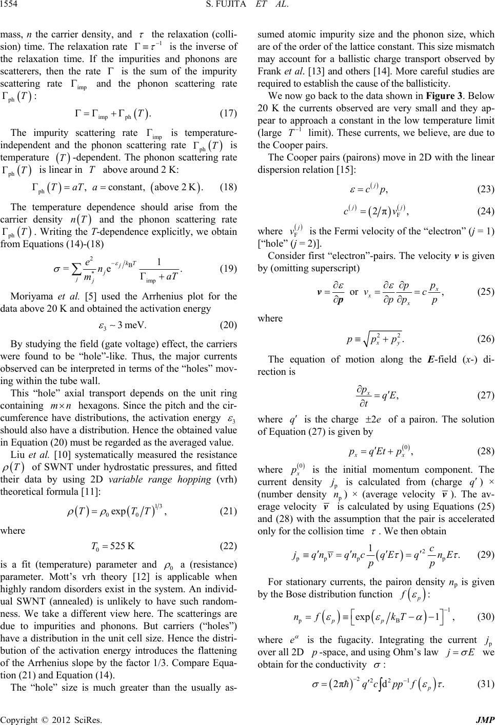

S. FUJITA ET AL.

1554

mass, n the carrier density, and



the relaxation (colli-

sion) time. The relaxation rate 1











ph .T

is the inverse of

the relaxation time. If the impurities and phonons are

scatterers, then the rate is the sum of the impurity

scattering rate

and the phonon scattering rate

: imp





imp





ph T

(17)

The impurity scattering rate imp is temperature-

independent and the phonon scattering rate





ΓT



 

above2K

ph is

temperature -dependent. The phonon scattering rate

is linear in above around 2 K:



Taa







ph T



ph T



Γconstant,,T



. (18)

The temperature dependence should arise from the

carrier density and the phonon scattering rate

. Writing the T-dependence explicitly, we obtain

from Equations (14)-(18)

imp

naT







33meV

(19)





Moriyama et al. [5] used the Arrhenius plot for the

data above 20 K and obtained the activation energy





n

(20)

By studying the field (gate voltage) effect, the carriers

were found to be “hole”-like. Thus, the major currents

observed can be interpreted in terms of the “holes” mov-

ing within the tube wall.

This “hole” axial transport depends on the unit ring

containing hexagons. Since the pitch and the cir-

cumference have distributions, the activation energy 3



should also have a distribution. Hence the obtained value

in Equation (20) must be regarded as the averaged value.

Liu et al. [10] systematically measured the resistance

of SWNT under hydrostatic pressures, and fitted

their data by using 2D variable range hopping (vrh)

theoretical formula [11]:







exp ,TT

0525 KT



 (21)

where

(22)

is a fit (temperature) parameter and 0



a (resistance)

parameter. Mott’s vrh theory [12] is applicable when

highly random disorders exist in the system. An individ-

ual SWNT (annealed) is unlikely to have such random-

ness. We take a different view here. The scatterings are

due to impurities and phonons. But carriers (“holes”)

have a distribution in the unit cell size. Hence the distri-

bution of the activation energy introduces the flattening

of the Arrhenius slope by the factor 1/3. Compare Equa-

tion (21) and Equation (14).

The “hole” size is much greater than the usually as-

sumed atomic impurity size and the phonon size, which

are of the order of the lattice constant. This size mismatch

may account for a ballistic charge transport observed by

Frank et al. [13] and others [14]. More careful studies are

required to establish the cause of the ballisticity.

We now go back to the data shown in Figure 3. Below

20 K the currents observed are very small and they ap-

pear to approach a constant in the low temperature limit

(large 1



limit). These currents, we believe, are due to

the Cooper pairs.

The Cooper pairs (pairons) move in 2D with the linear

dispersion relation [15]:









(23)



2π,

cv



(24)

where



v is the Fermi velocity of the “electron” (j = 1)

[“hole” (j = 2)].

Consider first “electron”-pairs. The velocity v is given

by (omitting superscript)

or ,

pp p









vp (25)

where

ppp (26)

The equation of motion along the E-field (x-) di-

rection is

pqE







(27)



is the charge 2e

where



of a pairon. The solution

of Equation (27) is given by



pqEtp







(28)

where

p is the initial momentum component. The

current density

jq is calculated from (charge



) ×

(number density

n) × (average velocity v). The av-

erage velocity v is calculated by using Equations (25)

and (28) with the assumption that the pair is accelerated

only for the collision time



. We then obtain



pp pp

jqnvqncqEqnE



 

 



(29)

For stationary currents, the pairon density np is given

by the Bose distribution function f



 

exp1 ,

nf kT









 

(30)







is the fugacity. Integrating the current

where j

pjE

over all 2D -space, and using Ohm’s law





obtain for the conductivity





222 1

2πd.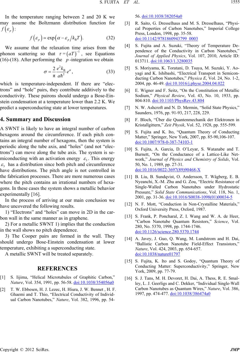

qcpp f









 (31)



S. FUJITA ET AL.

1555



In the temperature ranging between 2 and 20 K we

may assume the Boltzmann distribution function for



 

exp







=aT





 (32)

We assume that the relaxation time arises from the

phonon scattering so that , see Equations

(16)-(18). After performing the -integration we obtain

ek e





 (33)

which is temperature-independent. If there are “elec-

trons” and “hole” pairs, they contribute additively to the

conductivity. These pairons should undergo a Bose-Ein-

stein condensation at a temperature lower than 2.2 K. We

predict a superconducting state at lower temperatures.

4. Summary and Discussion

A SWNT is likely to have an integral number of carbon

hexagons around the circumference. If each pitch con-

tains an integral number of hexagons, then the system is

periodic along the tube axis, and “holes” (and not “elec-

trons”) can move along the tube axis. The system is se-

miconducting with an activation energy 3



. This energy



has a distribution since both pitch and circumference

have distributions. The pitch angle is not controlled in

the fabrication processes. There are more numerous cases

where the pitch contains an irrational numbers of hexa-

gons. In these cases the system shows a metallic behavior

experimentally [16].

In the process of arriving at our main conclusion we

have uncovered the following results.

1) “Electrons” and “holes” can move in 2D in the car-

bon wall in the same manner as in graphene.

2) For a metallic SWNT 1) implies that the conduction

in the wall shows no pitch dependence.

3) The Cooper pairs are formed in the wall. They

should undergo Bose-Einstein condensation at lower

temperature, exhibiting a superconducting state.

A metallic SWNT will be treated separately.

REFERENCES

[1] S. Iijima, “Helical Microtubules of Graphitic Carbon,”

Nature, Vol. 354, 1991, pp. 56-58. doi:10.1038/354056a0

[2] T. W. Ebbesen, H. J. Lezec, H. Hiura, J. W. Bennet , H. F.

Ghaemi and T. Thio, “Electrical Conductivity of Individ-

ual Carbon Nanotubes,” Nature, Vol. 382, 1996, pp. 54-

56. doi:10.1038/382054a0

[3] R. Saito, G. Dresselhaus and M. S. Dresselhaus, “Physi-

cal Properties of Carbon Nanotubes,” Imperial College

Press, London, 1998, pp. 35-58.

doi:10.1142/9781860943799_0003

[4] S. Fujita and A. Suzuki, “Theory of Temperature De-

pendence of the Conductivity in Carbon Nanotubes,”

Journal of Applied Physics, Vol. 107, 2010, Article ID:

013711. doi:10.1063/1.3280035

[5] S. Moriyama, K. Toratani, D. Tsuya, M. Suzuki, Y. Ao-

yagi and K. Ishibashi, “Electrical Transport in Semicon-

ducting Carbon Nanotubes,” Physica E, Vol. 24, No. 1-2,

2004, pp. 46-49. doi:10.1016/j.physe.2004.04.022

[6] E. Wigner and F. Seitz, “On the Constitution of Metallic

Sodium,” Physical Review, Vol. 43, No. 10, 1933, pp.

804-810. doi:10.1103/PhysRev.43.804

[7] N. W. Ashcroft and N. D. Mermin, “Solid State Physics,”

Saunders, 1976, pp. 91-93, 217, 228, 229.

[8] F. Bloch, “Über die Quantenmechanik der Elektronen in

Kristallgittern,” Z eit Physik, Vol. 52, 1928, pp. 555-599.

[9] S. Fujita and K. Ito, “Quantum Theory of Conducting

Matter,” Springer, New York, 2007, pp. 85-90,106-107.

doi:10.1007/978-0-387-74103-1

[10] S. Fujita, A. Garcia, D. O’Leyar, S. Watanabe and T.

Burnett, “On the Conductance of a Lattice-Like Net-

work,” Journal of Physics and Chemistry of Solids, Vol.

50, No. 1, 1989, pp. 27-31.

doi:10.1016/0022-3697(89)90468-X

[11] B. Liu, B. Sundqvist, O. Andersson, T. Wågberg, E. B.

Nyeanchi, X.-M. Zhu and G. Zou, “Electric Resistance of

Single-Walled Carbon Nanotubes under Hydrostatic

Pressure,” Solid State Communications, Vol. 118, No. 1,

2001, pp. 31-36. doi:10.1016/S0038-1098(01)00034-5

[12] N. F. Mott, “Conduction in Non-Crystalline Materials,”

Oxford University Press, Oxford, 1987.

[13] S. Frank, P. Poncharal, Z. I. Wang and W. A. de Heer,

“Carbon Nanotube Quantum Resistors,” Science, Vol.

280, No. 5370, 1998, pp. 1744-1746.

doi:10.1126/science.280.5370.1744

[14] A. Javey, J. Guo, Q. Wang, M. Lundstrom and H. Dai,

“Ballistic Carbon Nanotube Field-Effect Transistors,”

Nature, Vol. 424, 2003, pp. 654-657.

doi:10.1038/nature01797

[15] S. Fujita, K. Ito and S. Godoy, “Quantum Theory of

Conducting Matter: Superconductivity,” Springer, New

York, 2009, pp. 77-79.

[16] S. J. Tans, M. H. Devoret, H. Dai, A. Thess, R. E. Smal-

ley, L. J. Geerligs and C. Dekker, “Individual Single-Wall

Carbon Nanotubes as Quantum Wires,” Nature, Vol. 386,

1997, pp. 474-477. doi:10.1038/386474a0