Hydraulic Jump in the Gulf of California

doi:10.4236/ojms.2012.24017

Paper Menu >>

Journal Menu >>

Open Journal of Marine Science, 2012, 2, 141-149

http://dx.doi.org/10.4236/ojms.2012.24017 Published Online October 2012 (http://www.SciRP.org/journal/ojms)

Hydraulic Jump in the Gulf of California

David Salas-Monreal1, David Alberto Salas-de-Leon2, María Adela Monreal-Gomez2,

Mayra Lorena Riverón-Enzástiga3, Erika Mojica-Ramírez3

1Instituto de Ciencias Marinas y Pesquerias, Universidad Veracruzana, Veracruz, Mexico

2Instituto de Ciencias del Mar y Limnología, Mexico City, Mexico

3Posgrado en Ciencias del Mar y Limnología, Mexico City, Mexico

Email: [email protected]

Received June 8, 2012; revised July 3, 2012; accepted August 1, 2012

ABSTRACT

Acoustic Doppler current profiles and water density profiles were measured over the 280 m deep continental slope of

the Gulf of California to elucidate the bathymetric effect on zooplankton distribution. These measurements were com-

bined with water velocity and density simulations from the Regional Ocean Model System with and without the influ-

ence of Coriolis acceleration. The data revealed an acceleration of the near-bottom flow as it moved toward increasing

depths. This acceleration was produced by the adjustment of the isopycnals to bathymetry (hydraulic jump). Zooplank-

ton patches moved downward at the continental slope and then upward, thus exhibiting wave patterns. Model outputs

without the effect of Coriolis acceleration also suggested that vertical zooplankton concentration followed a wave pat-

tern. However, when Coriolis acceleration was added to the momentum equation, the horizontal zooplankton distribu-

tion was enhanced, which reduced the vertical zooplankton concentration observed over irregular bathymetries. Coriolis

acceleration was responsible for horizontal dispersal of up to 20% of the total zooplankton concentration located over

the wave trough.

Keywords: Hydraulic Jump; Acoustic Doppler Current Profiles; Internal Waves; Zooplank ton Biovolumes; Gulf of

California

1. Introduction

An understanding of the stratified flow dynamics over

irregular bathymetries is crucial for predicting flow pat-

terns [1], lee wave generation [2], and their interactions

with planktonic and organic matter concentration [3-7].

Such interactions depend on the degree of stratification

and on the strength of tidal forcing [8]. Internal waves

generated over irregular bathymetries explain part of the

temperature and salinity variations observed in the water

column [2]. Therefore, the vertical variation of the py-

cnocline, where most particulate and dissolved organic

matter are concentrated [9], could be related to irregular

bathymetries such as the continental slope [10], subma-

rine canyons [7], and seamounts [11].

Increased vertical and horizontal nutrient flux occurs

in areas with abrupt bathymetric changes where internal

waves break and produce mixing and increase primary

productivity. For example, in Mon terey Bay, one-third of

the planktonic production was associated with amplified

internal wave activity caused by the bathymetry of the

Monterey Canyon [12]. Vertical and horizontal water ex-

change in areas with abrupt bathymetric changes is also

attributed to shear instability [13]. The vertical displace-

ment of high-nutrient deep-water enhanced by internal

wave activity has a major ecological impact in adjacent

waters [14,15]. Therefore, an understanding of current

velocities and vertical water density variations induced

by internal wave activity is crucial to describe near-sur-

face concentration of planktonic organisms, nutrients,

and detritus.

The amplification of internal waves over the con tinen-

tal slope are not commonly observed, therefore numeri-

cal models have described the near-surface concentration

of organisms over internal wave troughs [16]. The near-

surface distribution of planktonic organism over bathy-

metric changes is usually assumed to be related to cyc-

lonic eddies, nutrients, light penetration, and amplified

internal wave activity [17]. However, the asymmetry of

the water mass exchange is attributed to Coriolis accel-

eration [18]. The goal of this study is to advance our un-

derstanding of the distribution of zooplankton and its

dependence on amplified internal wave activity induced

by bathymetric changes such as the continental slope,

under the influence of Coriolis acceleration.

2. Data Collection and Processing

2.1. Data Collection

Current profiles and backscatter intensity data from an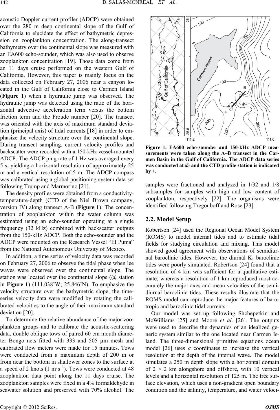

D. SALAS-MONREAL ET AL.

142

acoustic Doppler current profiler (ADCP) were obtained

over the 280 m deep continental slope of the Gulf of

California to elucidate the effect of bathymetric depres-

sion on zooplankton concentration. The along-transect

bathymetry over the continental slope was measured with

an EA600 echo-sounder, which was also used to observe

zooplankton concentration [19]. Those data come from

an 11 days cruise performed on the western Gulf of

California. However, this paper is mainly focus on the

data collected on February 27, 2006 near a canyon lo-

cated in the Gulf of California close to Carmen Island

(Figure 1) when a hydraulic jump was observed. The

hydraulic jump was detected using the ratio of the hori-

zontal advective acceleration term versus the bottom

friction term and the Froude number [20]. The transect

was oriented with the axis of maximum standard devia-

tion (principal axis) of tidal cu rrents [18] in order to em-

phasize the velocity structure over the continental slope.

During transect sampling, current velocity profiles and

backscatter were recorded with a 150-kHz vessel-mounted

ADCP. Th e ADCP ping rate of 1 Hz was avera ged every

5 s, yielding a horizontal resolution of approximately 25

m and a vertical resolution of 5 m. The ADCP compass

was calibrated using a global positioning system data set

following Trump and Marmorino [21].

The density profiles were obtained from a conductivity-

temperature-depth (CTD of the Niel Brown company,

version IV) along transect A-B (Figure 1). The concen-

tration of zooplankton within the water column was

estimated using an echo-sounder operating at a single

frequency (32 kHz) combined with backscatter outputs

from the 150-kHz ADCP. Both the echo-sounder and the

ADCP were mounted on the Research Vessel “El Puma”

from the National Autonomous University of Mexico.

In addition, a time series of velocity data was recorded

on February 27, 2006 to observe the tidal phase when lee

waves were observed over the continental slope. The

station was located over the continental slope (@ station

in Figure 1) (111.038˚W; 25.846˚N). To emphasize the

velocity structure over the bathymetric slope, the time-

series velocity data were modified by rotating the cali-

brated velocities to the angle of their maximum standard

deviatio n [ 2 0].

To determine the relative abundance of the major zoo-

plankton groups and to calibrate the acoustic-scattering

data, double oblique tows of paired 60 cm mouth diame-

ter Bongo nets fitted with 333 and 505 µm mesh and

calibrated flow meters were made for 15 minutes. Tows

were conducted from a maximum depth of 200 m or

from near the bottom in shallower zones to the surface at

a speed of 2 knots (1 m·s–1). Tows were conducted at 48

zooplankton data point along the 11 days cruise. The

zooplankton samples were fixed in a 4% formaldehyde in

seawater solution and preserved with 70% alcohol. The

Gulf of California

23N

31N

108 W

114 W

25.8 26.1

111.2111.0

Carmen Island

100

300

200

300

100

200

Figure 1. EA600 echo-sounder and 150-kHz ADCP mea-

surements were taken along the A–B transect in the Car-

men Basin in the Gulf of California. The ADCP data series

was conducted at @ and the CTD profile station is indicated

by +.

samples were fractioned and analyzed in 1/32 and 1/8

subsamples for samples with high and low content of

zooplankton, respectively [22]. The organisms were

identified following Tregouboff and Rose [23].

2.2. Model Setup

Robertson [24] used the Regional Ocean Model System

(ROMS) to model internal tides and to estimate tidal

fields for studying circulation and mixing. This model

showed good agreement with observations of semidiur-

nal baroclinic tides. However, the diurnal K1 baroclinic

tides were poorly simulated. Robertson [24] found that a

resolution of 4 km was sufficient for a qualitative esti-

mate; whereas a resolution of 1 km reproduced most ac-

curately the major axes and mean velocities of the semi-

diurnal baroclinic tides. These results illustrate that the

ROMS model can reproduce the major features of baro-

tropic and baroclinic tidal currents.

Our model was set up following Shchepetkin and

McWilliams [25] and Moore et al. [26]. The outputs

were used to describe the dynamics of an idealized ge-

neric system similar to the one located near Carmen Is-

land. The three-dimensional primitive equations ocean

model [26] uses σ coordinates to increase the vertical

resolution at the depth of the internal wave. The model

simulates a 250 m depth slope with a horizontal domain

of 2 × 2 km alongshore and offshore, with 10 vertical

levels and a horizontal resolution of 125 m. The free sur-

face elevation, which uses a non-gradient open boundary

condition and the salinity, temperature, and water velo ci-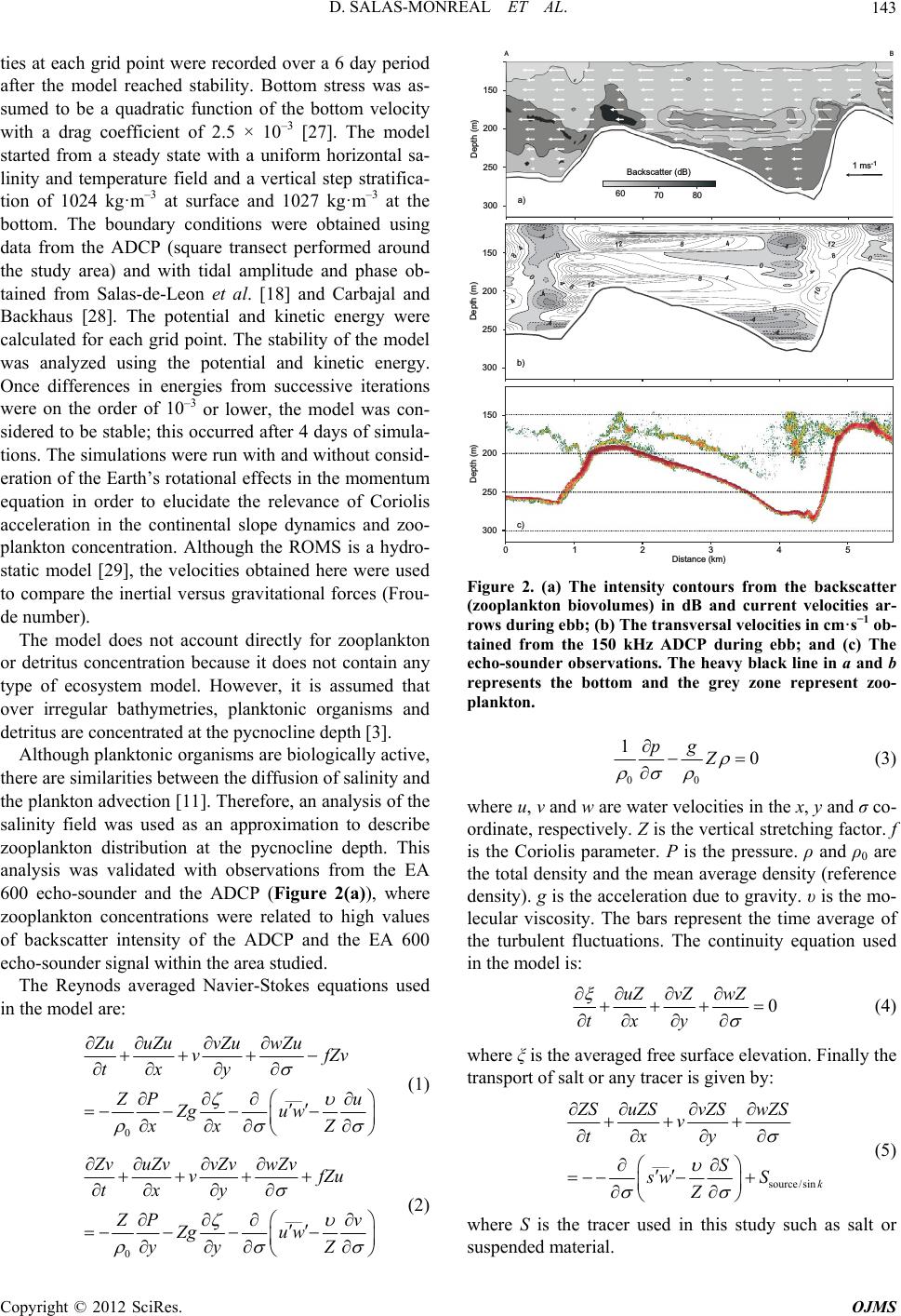

D. SALAS-MONREAL ET AL. 143

ties at each grid point were recorded over a 6 day period

after the model reached stability. Bottom stress was as-

sumed to be a quadratic function of the bottom velocity

with a drag coefficient of 2.5 × 10–3 [27]. The model

started from a steady state with a uniform horizontal sa-

linity and temperature field and a vertical step stratifica-

tion of 1024 kg·m–3 at surface and 1027 kg·m–3 at the

bottom. The boundary conditions were obtained using

data from the ADCP (square transect performed around

the study area) and with tidal amplitude and phase ob-

tained from Salas-de-Leon et al. [18] and Carbajal and

Backhaus [28]. The potential and kinetic energy were

calculated for each grid point. The stability of the model

was analyzed using the potential and kinetic energy.

Once differences in energies from successive iterations

were on the order of 10–3 or lower, the model was con-

sidered to be stable; this occurred after 4 days of simula-

tions. The simulation s were run with and without consid-

eration of the Earth’s rotational effects in the momentum

equation in order to elucidate the relevance of Coriolis

acceleration in the continental slope dynamics and zoo-

plankton concentration. Although the ROMS is a hydro-

static model [29], the velocities obtained here were used

to compare the inertial versus gravitational forces (Frou-

de number).

The model does not account directly for zooplankton

or detritus concentration because it does not contain any

type of ecosystem model. However, it is assumed that

over irregular bathymetries, planktonic organisms and

detritus are concentrated at the pycnocline depth [3].

Although planktonic organisms are biologically active,

there are similarities between the diffusion of salinity and

the plankton advection [11]. Therefore, an analysis of the

salinity field was used as an approximation to describe

zooplankton distribution at the pycnocline depth. This

analysis was validated with observations from the EA

600 echo-sounder and the ADCP (Figure 2(a)), where

zooplankton concentrations were related to high values

of backscatter intensity of the ADCP and the EA 600

echo-sounder signal within the area studied.

The Reynods averaged Navier-Stokes equations used

in the model are:

___

Zu uZuvZu wZu

tx yZv

Zgu w

xx Z









 

 

 





 



 



(1)

___

Zv uZvvZv wZv

tx y

-4

1ms

-1

Backscatter (dB)

150

200

250

300

Depth (m)

60 80

A B

12345

Distance (km)

150

200

250

300

Depth (m)

150

200

250

300

Depth (m)

Figure 2. (a) The intensity contours from the backscatter

(zooplankton biovolumes) in dB and current velocities ar-

rows during ebb; (b) The transversal velocities in cm·s−1 ob-

tained from the 150 kHz ADCP during ebb; and (c) The

echo-sounder observations. The heavy black line in a and b

represents the bottom and the grey zone represent zoo-

plankton.











 (3)

where u, v and w are water velocities in the x, y and σ co-

ordinate, respectively. Z is the vertical stretching factor. f

is the Coriolis parameter. P is the pressure. ρ and ρ0 are

the total density and the mean average density (reference

density). g is the acceleration due to gravity. υ is the mo-

lecular viscosity. The bars represent the time average of

the turbulent fluctuations. The continuity equation used

in the model is:

uZ vZ wZ

tx y





 



 

  (4)

where ξ is the averaged free surface elevation. Finally the

transport of salt or any tracer is given by:

___

source/sin k

ZS uZSvZS wZS

tx y

sw S











 

 







 







(5)

Zgu w

yy Z









 

 

 





 



 



(2) where S is the tracer used in this study such as salt or

suspended material.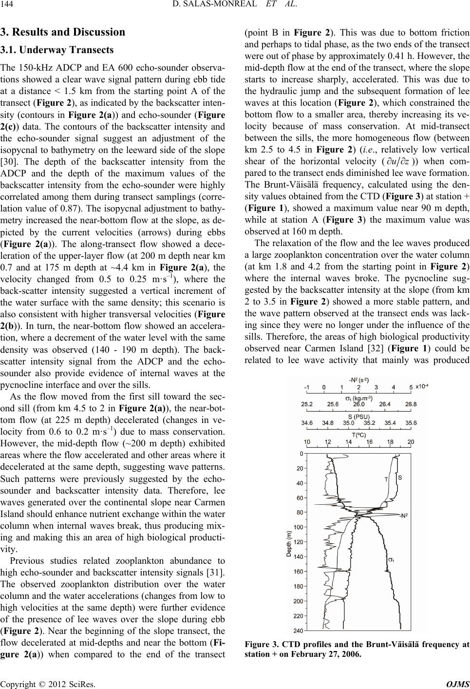

D. SALAS-MONREAL ET AL.

144

3. Results and Discussion

3.1. Underway Transects

The 150-kHz ADCP and EA 600 echo-sounder observa-

tions showed a clear wave signal pattern during ebb tide

at a distance < 1.5 km from the starting point A of the

transect (Figure 2), as indicated by the backscatter inten-

sity (contours in Figure 2(a)) and echo-sounder (Figure

2(c)) data. The contours of the backscatter intensity and

the echo-sounder signal suggest an adjustment of the

isopycnal to bathymetry on the leeward side of the slope

[30]. The depth of the backscatter intensity from the

ADCP and the depth of the maximum values of the

backscatter intensity from the echo-sounder were highly

correlated among them during transect samplings (corre-

lation value of 0.87). The isopycnal adjustment to bathy-

metry increased the near-bo ttom flow at the slope, as de-

picted by the current velocities (arrows) during ebbs

(Figure 2(a)). The along-transect flow showed a dece-

leration of the upper-layer flow (at 200 m depth near km

0.7 and at 175 m depth at ~4.4 km in Figure 2(a), the

velocity changed from 0.5 to 0.25 m·s–1), where the

back-scatter intensity suggested a vertical increment of

the water surface with the same density; this scenario is

also consistent with higher transversal velocities (Figure

2(b)). In turn, the near-bottom flow showed an accelera-

tion, where a decrement of the water level with the same

density was observed (140 - 190 m depth). The back-

scatter intensity signal from the ADCP and the echo-

sounder also provide evidence of internal waves at the

pycnocline interface and over the sills.

As the flow moved from the first sill toward the sec-

ond sill (from km 4.5 to 2 in Figure 2(a)), the near-bot-

tom flow (at 225 m depth) decelerated (changes in ve-

locity from 0.6 to 0.2 m·s–1) due to mass conservation.

However, the mid-depth flow (~200 m depth) exhibited

areas where the flow accelerated and other areas where it

decelerated at the same depth, suggesting wave patterns.

Such patterns were previously suggested by the echo-

sounder and backscatter intensity data. Therefore, lee

waves generated over the continental slope near Carmen

Island should enhance nutrient exchange within the water

column when internal waves break, thus producing mix-

ing and making this an area of high biological producti-

vity.

Previous studies related zooplankton abundance to

high echo-sounder and backscatter intensity signals [31].

The observed zooplankton distribution over the water

column and the water accelerations (changes from low to

high velocities at the same depth) were further evidence

of the presence of lee waves over the slope during ebb

(Figure 2). Near the beginning of the slope transect, the

flow decelerated at mid-depths and near the bottom (Fi-

gure 2(a)) when compared to the end of the transect

(point B in Figure 2). This was due to bottom friction

and perhaps to tidal ph ase, as the two ends of the transect

were out of phase by approximately 0.41 h. However, the

mid-depth flow at the end of the transect, where the slope

starts to increase sharply, accelerated. This was due to

the hydraulic jump and the subsequent formation of lee

waves at this location (Figure 2), which constrained the

bottom flow to a smaller area, thereby increasing its ve-

locity because of mass conservation. At mid-transect

between the sills, the more homogeneous flow (between

km 2.5 to 4.5 in Figure 2) (i.e., relatively low vertical

shear of the horizontal velocity (uz)) when com-

pared to the transect ends diminished lee wave formation.

The Brunt-Väisälä frequency, calculated using the den-

sity values obtained from the CTD (Figure 3) at station +

(Figure 1), showed a maximum value near 90 m depth,

while at station A (Figure 3) the maximum value was

observed at 160 m depth.

The relaxation of the flow and the lee waves produced

a large zooplankton concentration over the water column

(at km 1.8 and 4.2 from the starting point in Figure 2)

where the internal waves broke. The pycnocline sug-

gested by the backscatter intensity at the slope (from km

2 to 3.5 in Figure 2) showed a more stable pattern, and

the wave pattern observed at the transect ends was lack-

ing since they were no longer under the influence of the

sills. Therefore, the areas of high biological productivity

observed near Carmen Island [32] (Figure 1) could be

related to lee wave activity that mainly was produced

Figure 3. CTD profiles and the Brunt-Väisälä frequency at

station + on February 27, 2006.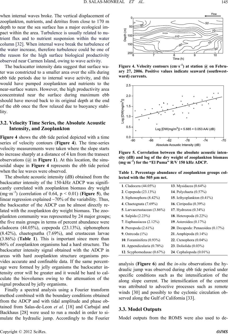

D. SALAS-MONREAL ET AL. 145

when internal waves broke. The vertical displacement of

zooplankton, nutrients, and detritus from close to 170 m

depth to near the sea surface has a major ecological im-

pact within the area. Turbulence is usually related to nu-

trient flux and to nutrient suspension within the water

column [32]. When internal wave break the turbulence of

the water increase, therefore turbulence could be one of

the reason for the high surface biological productivity

observed near Carmen Island, owing to wave activity.

The backscatter intensity data suggest that surface wa-

ter was constricted to a smaller area over the sills during

ebb tide periods due to internal wave activity, and this

would have pumped zooplankton and nutrients to the

near-surface waters. However, the high productivity area

concentrated near the surface during maximum ebb

should have moved back to its original depth at the end

of the ebb once the flow relaxed due to buoyancy stabi-

lity.

3.2. Velocity Time Series, the Absolute Acoustic

Intensity, and Zooplankton

Figure 4 shows the ebb tide period depicted with a time

series of velocity contours (Figure 4). The time-series

velocity measurements were taken where the slope starts

to increase sharply at a distance of 4 km from the transect

observations (@ in Figure 1). At this location, the sinu-

soidal shape in Figure 4 represents the ebb tide period

when the lee waves were observed.

The absolute aco ustic intensity (dB) obtained from the

backscatter intensity of the 150-kHz ADCP was signifi-

cantly correlated with zooplankton biomass dry weight

(mg·m–3) (correlation of 0.64, p < 0.01) (Figure 5), the

linear regression explained ~70% of the variability. Thus,

the backscatter of the ADCP can be almost directly re-

lated with the zooplankton dry weight b iomass. The zoo-

plankton community was represented by 24 major groups;

the five main groups in terms of percent abundance were

cladocera (44.05%), copepoda (23.13%), siphonophora

(8.42%), chaetognatha (7.69%), and crustacean larvae

(3.86%) (Table 1). This is important since more than

86% of zooplankton organisms had a hard structure. The

backscatter intensity signal obtained with the ADCP in

areas with hard zooplankton structure organisms pro-

vides accurate and confinable data. If the same percent-

age were formed by jelly organisms the backscatter in-

tensity error will be greater and it would be hard to cal-

culate the biovolumes owing to the attenuation of the

signal produced by jelly organisms.

Finally a spectral analysis using a Fourier transform

method combined with the boundary conditions obtained

from the ADCP and with tidal amplitude and phase ob-

tained from Salas-de-Leon et al. [18] and Carbajal and

Backhaus [28] were used to run a model in order to si-

mulate the hydraulic jump. Accordingly to the Fourier

9 108

100

150

200

Depth (m)

Time(h)

110

Flow

Figure 4. Velocity contours (cm·s–1) at station @ on Febru-

ary 27, 2006. Positive values indicate seaward (southwest-

ward) currents.

Log [DW(mg/m)]= 5.685 + 0.053

3AAI (dB)

0.0

0.5

1.0

1.5

2.0

2.5

-90 -86-82 -78-74 -70

Log [DW(mg/m)]

AbsoluteAcoustic Intensity (dB)

Figure 5. Correlation between the absolute acoustic inten-

sity (dB) and log of the dry weight of zooplankton biomass

(mg·m–3) for the “El Puma” R/V 150 kHz ADCP.

Table 1. Percentage abundance of zooplankton groups col-

lected with the 505 µm net.

1. Cladocera (44.05%) 13. Mysidacea (0.64%)

2. Copepoda (23 .13%) 14. Polychaeta (0.57%)

3. Siphonopho ra (8.42%) 15. Icthyop l ankton (0.41%)

4. Chaetognata (7.69%) 16. Cirripedia (0.39%)

5. Larvaecrustacean (3.86%)17. Hydrozoa (0.34%)

6. Salpida (2.23%) 18. Heteropoda (0.22%)

7. Euphausiacea (2.12%) 19. Asteroidea (0.17%)

8. Pteropoda (2.61%) 20. Decapoda: Penaeoidea ( 0. 17%)

9. Ostrcoda (1%) 21. Amphipoda (0.14%)

10. Foraminifera (0.93%) 22. Ctenophora (0.04%)

11. Appendicularia (0.78%) 23. Doliolida (0.03%)

12. Scyphomedusae (0.67%)24. Cepha lopoda (0.01%)

analysis (Figure 6) and the in-situ observations the hy-

draulic jump was observed during ebb tide period under

specific conditions such as the intensification of the

along slope current. The intensification of the current

was attributed to advective processes such as remote

winds [30] and possibly to the cyclonic circulation ob-

served along the Gulf of California [33].

3.3. Model Outputs

Model outputs from the ROMS were also used to de-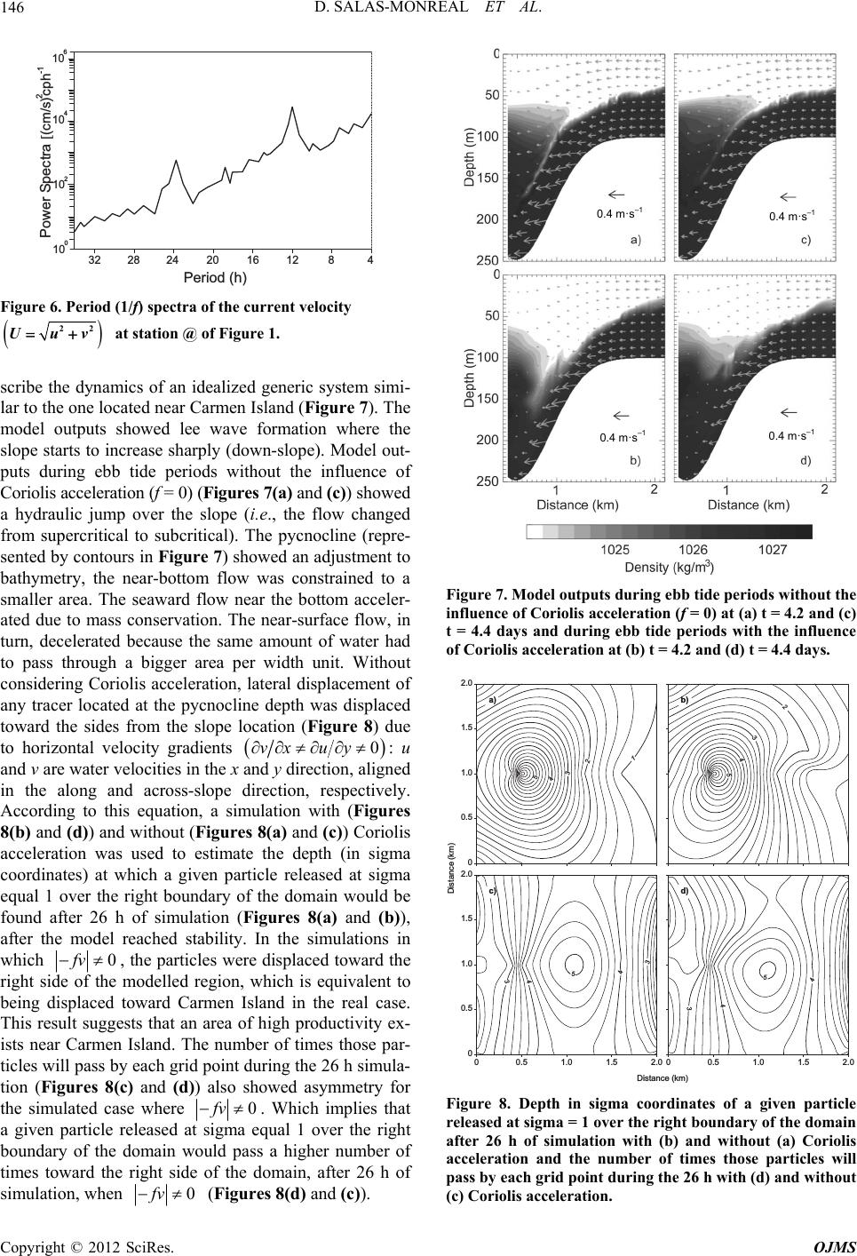

D. SALAS-MONREAL ET AL.

146

Power Spectra

[(cm/s) cph

2-1

Period (h)

10 32 28 24 20 16 1284

102

Figure 6. Period (1/f) spectra of the current velocity





Uuv

at station @ of Figure 1.

scribe the dynamics of an idealized generic system simi-

lar to the one located near Carmen Island (Figure 7). The

model outputs showed lee wave formation where the

slope starts to increase sharp ly (down-slope). Model out-

puts during ebb tide periods without the influence of

Coriolis acceleration (f = 0) (Figures 7(a) and (c)) sho w ed

a hydraulic jump over the slope (i.e., the flow changed

from supercritical to subcritical). The pycnocline (repre-

sented by contours in Figure 7) showed an adjustment to

bathymetry, the near-bottom flow was constrained to a

smaller area. The seaward flow near the bottom acceler-

ated due to mass conservation. The near-surface flow, in

turn, decelerated because the same amount of water had

to pass through a bigger area per width unit. Without

considering Coriolis acceleration, lateral displacement of

any tracer located at the pycnocline depth was displaced

toward the sides from the slope location (Figure 8) due

to horizontal velocity gradients



0vxuy : u

and v are water velocities in the x and y direction, aligned

in the along and across-slope direction, respectively.

According to this equation, a simulation with (Figures

8(b) and (d)) and without (Figures 8(a) and (c)) Coriolis

acceleration was used to estimate the depth (in sigma

coordinates) at which a given particle released at sigma

equal 1 over the right boundary of the domain would be

found after 26 h of simulation (Figures 8(a) and (b)),

after the model reached stability. In the simulations in

which 0fv, the particles were displaced toward the

right side of the modelled region, which is equivalent to

being displaced toward Carmen Island in the real case.

This result suggests that an area of high productivity ex-

ists near Carmen Island. The number of times those par-

ticles will pass by each grid point during the 26 h simula-

tion (Figures 8(c) and (d)) also showed asymmetry for

the simulated case where 0fv. Which implies that

a given particle released at sigma equal 1 over the right

boundary of the domain would pass a higher number of

times toward the right side of the domain, after 26 h of

simulation, when 0fv

(Figures 8(d) and (c)).

0.4 m·s

–1

0.4 m·s

–1

0.4 m·s

–1

0.4 m·s

–1

Figure 7. Model outputs during ebb tide periods without the

influence of Coriolis acceleration (f = 0) at (a) t = 4.2 and (c)

t = 4.4 days and during ebb tide periods with the influence

of Coriolis acceleration at (b) t = 4.2 and (d) t = 4.4 days.

0.5

1.0

1.5

2.0

00.5 1.0 1.5 2.0

0.5

1.0

1.5

2.0

00.5 1.0 1.5 2.0

Distance (km)

a) b)

c) d)

Figure 8. Depth in sigma coordinates of a given particle

released at sigma = 1 over the right boundary of the domain

after 26 h of simulation with (b) and without (a) Coriolis

acceleration and the number of times those particles will

pass by each grid point during the 26 h with (d) and without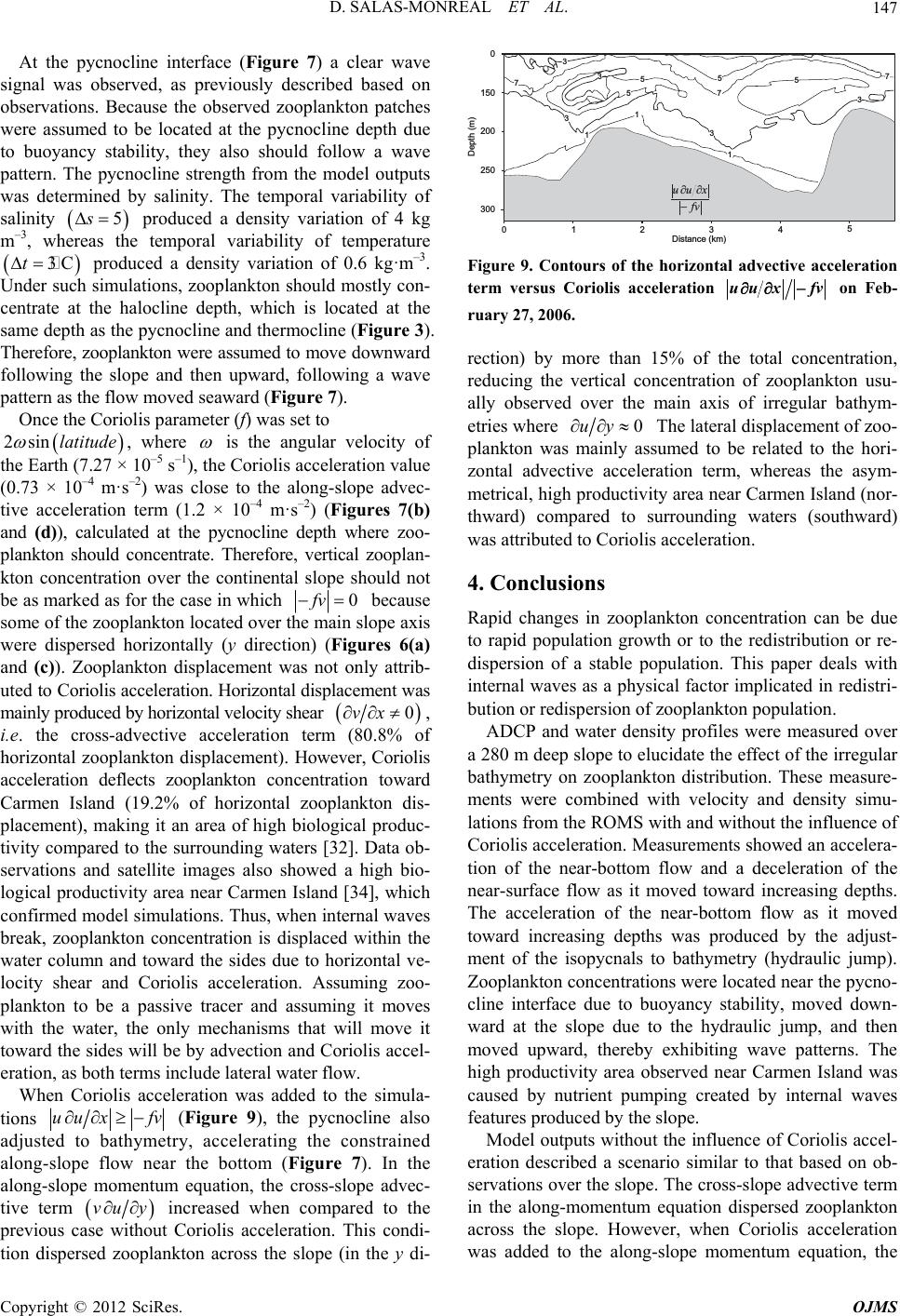

D. SALAS-MONREAL ET AL. 147

At the pycnocline interface (Figure 7) a clear wave

signal was observed, as previously described based on

observations. Because the observed zooplankton patches

were assumed to be located at the pycnocline depth due

to buoyancy stability, they also should follow a wave

pattern. The pycnocline strength from the model outputs

was determined by salinity. The temporal variability of

salinity produced a density variation of 4 kg

m–3, whereas the temporal variability of temperature

produced a density variation of 0.6 kg·m–3.

Under such simulations, zooplank ton should mostly con-

centrate at the halocline depth, which is located at the

same depth as the pycnocline and thermocline (Figure 3).

Therefore, zooplankton were assumed to move d ownw ard

following the slope and then upward, following a wave

pattern as the flow moved seaward (Figure 7).



5s





t

Once the Coriolis parameter (f) was set to

, where



2sinlatitude



is the angular velocity of

the Earth (7.27 × 10–5 s–1), the Coriolis acceleration value

(0.73 × 10–4 m·s–2) was close to the along-slope advec-

tive acceleration term (1.2 × 10–4 m·s–2) (Figures 7(b)

and (d)), calculated at the pycnocline depth where zoo-

plankton should concentrate. Therefore, vertical zooplan-

kton concentration over the continental slope should not

be as marked as for the case in which 0fv because

some of the zooplankton located over the main slope axis

were dispersed horizontally (y direction) (Figures 6(a)

and (c)). Zooplankton displacement was not only attrib-

ute d to Coriolis acceleration. Horizontal displacement was

mainly produced by horizontal velocity shear



0vx



i.e. the cross-advective acceleration term (80.8% of

horizontal zooplankton displacement). However, Coriolis

acceleration deflects zooplankton concentration toward

Carmen Island (19.2% of horizontal zooplankton dis-

placement), making it an area of high biological produc-

tivity compared to the surrounding waters [32]. Data ob-

servations and satellite images also showed a high bio-

logical productivity area near Carmen Island [34], which

confirmed model simulations. Thus, when internal waves

break, zooplankton concentration is displaced within the

water column and toward the sides due to horizontal ve-

locity shear and Coriolis acceleration. Assuming zoo-

plankton to be a passive tracer and assuming it moves

with the water, the only mechanisms that will move it

toward the sides will be by advection and Coriolis accel-

eration, as both terms include lateral water flow.

When Coriolis acceleration was added to the simula-

tions uu xfv (Figure 9), the pycnocline also

adjusted to bathymetry, accelerating the constrained

along-slope flow near the bottom (Figure 7). In the

along-slope momentum equation, the cross-slope advec-

tive term



vu y

150

200

250

300

Depth (m)

12345

Distance (km)

xuu

¶¶

Figure 9. Contours of the horizontal advective acceleration

term versus Coriolis acceleration uu x

v  on Feb-

ruary 27, 2006.

rection) by more than 15% of the total concentration,

reducing the vertical concentration of zooplankton usu-

ally observed over the main axis of irregular bathym-

etries where 0uy



 The lateral displacement of zoo-

plankton was mainly assumed to be related to the hori-

zontal advective acceleration term, whereas the asym-

metrical, high productivity area n ear Carmen Island (nor-

thward) compared to surrounding waters (southward)

was attributed to Coriolis acceleration.

4. Conclusions

Rapid changes in zooplankton concentration can be due

to rapid population growth or to the redistribution or re-

dispersion of a stable population. This paper deals with

internal waves as a physical factor implicated in redistri-

bution or redispersion of zooplankton population.

ADCP and water density profiles were measured over

a 280 m deep slope to elucidate the effect of the irregular

bathymetry on zooplankton distribution. These measure-

ments were combined with velocity and density simu-

lations from the ROMS with and without the influence of

Coriolis acceleration. Measurements showed an accelera-

tion of the near-bottom flow and a deceleration of the

near-surface flow as it moved toward increasing depths.

The acceleration of the near-bottom flow as it moved

toward increasing depths was produced by the adjust-

ment of the isopycnals to bathymetry (hydraulic jump).

Zooplankton concentrations were located near the pycno-

cline interface due to buoyancy stability, moved down-

ward at the slope due to the hydraulic jump, and then

moved upward, thereby exhibiting wave patterns. The

high productivity area observed near Carmen Island was

caused by nutrient pumping created by internal waves

features produced by the slope.

Model outputs without the influence of Coriolis accel-

eration described a scenario similar to that based on ob-

servations over the slope. The cross-slope advective term

in the along-momentum equation dispersed zooplankton

across the slope. However, when Coriolis acceleration

was added to the along-slope momentum equation, the



increased when compared to the

previous case without Coriolis acceleration. This condi-

tion dispersed zooplankton across the slope (in the y di-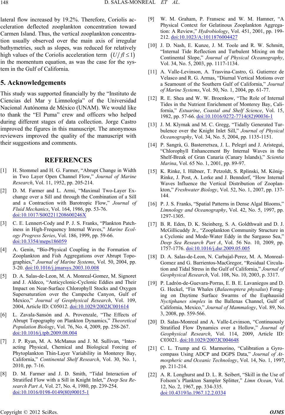

D. SALAS-MONREAL ET AL.

148

lateral flow increased by 19.2%. Therefore, Coriolis ac-

celeration deflected zooplankton concentration toward

Carmen Island. Thus, the vertical zooplankton concentra-

tion usually observed over the main axis of irregular

bathymetries, such as slopes, was reduced for relatively

high values of the Coriolis acceleration term



1Ufl



in the momentum equation, as was the case for the sys-

tem in the Gulf of California.

5. Acknowledgements

This study was supported financially by the “Instituto de

Ciencias del Mar y Limnología” of the Universidad

Nacional Autónoma de México (UNAM). We would like

to thank the “El Puma” crew and officers who helped

during different stages of data collection. Jorge Castro

improved the figures in this manuscript. The anonymous

reviewers improved the quality of the manuscript with

their suggestions and comments.

REFERENCES

[1] H. Stommel and H. G. Farmer, “Abrupt Change in Width

in Two Layer Open Channel Flow,” Journal of Marine

Research, Vol. 11, 1952, pp. 205-214.

[2] D. M. Farmer and L. Armi, “Maximal Two-Layer Ex-

change over a Sill and through the Combination of a Sill

and a Contraction with Barotropic Flow,” Journal of

Fluid Mechanics, Vol. 164, 1986, pp. 53-76.

doi:10.1017/S002211208600246X

[3] C. E. Lennert-Cody and P. J. S. Franks, “Plankton Patch-

iness in High-Frequency Internal Waves,” Marine Ecol-

ogy Progress Series, Vol. 186, 1999, pp. 59-66.

doi:10.3354/meps186059

[4] A. Genin, “Bio-Physical Coupling in the Formation of

Zooplankton and Fish Aggregations over Abrupt Topo-

graphies,” Journal of Marine Systems, Vol. 50, 2004, pp.

3-20. doi:10.1016/j.jmarsys.2003.10.008

[5] D. A. Salas-de-Leon, M. A. Monreal-Gomez, M. Signoret

and J. Aldeco, “Anticyclonic-Cyclonic Eddies and Their

Impact on Near-Surface Chlorophyll Stocks and Oxygen

Supersaturation over the Campeche Canyon, Gulf of

Mexico,” Journal of Geophysical Research, Vol. 109,

2004, Article ID: C05012. doi:10.1029/2002JC001614

[6] L. Zavala-Sansón and A. Provenzale, “The Effects of

Abrupt Topography on Plankton Dynamics,” Theoretical

Population Biology, Vol. 76, No. 4, 2009, pp. 258-267.

doi:10.1016/j.tpb.2009.08.004

[7] J. P. Ryan, M. A. McManus and J. M. Sullivan, “Inter-

acting Physical, Chemical and Biological Forcing of

Phytoplankton Thin-Layer Variability in Monterey Bay,

California,” Continental Shelf Research, Vol. 30, No. 1,

2010, pp. 7-16.

[8] D. M. Farmer and J. D. Smith, “Tidal Interaction of

Stratified Flow with a Sill in Knight Inlet,” Deep Sea Re-

search Part A, Vol. 27, No. 4, 1980, pp. 239-254.

doi:10.1016/0198-0149(80)90015-1

[9] W. M. Graham, P. Fransesc and W. M. Hamner, “A

Physical Context for Gelatinous Zooplankton Aggrega-

tion: A Review,” Hydrobiology, Vol. 451, 2001, pp. 199-

212. doi:10.1023/A:1011876004427

[10] J. D. Nash, E. Kunze, J. M. Toole and R. W. Schmitt,

“Internal Tide Reflection and Turbulent Mixing on the

Continental Slope,” Journal of Physical Oceanography,

Vol. 34, No. 5, 2003, pp. 1117-1134.

[11] A. Valle-Levinson, A. Trasvina-Castro, G. Gutierrez de

Velasco a n d R. G. Armas, “Diurnal Vertical Motions over

a Seamount of the Southern Gulf of California,” Journal

of Marine Systems, Vol. 50, No. 1, 2004, pp. 61-77.

[12] R. E. Shea and W. W. Broenkow, “The Role of Internal

Tides in the Nutrient Enrichment of Monterey Bay, Cali-

fornia,” Estuarine, Coastal and Shelf Science, Vol. 15,

1982, pp. 57-66. doi:10.1016/0272-7714(82)90036-1

[13] J. M. Klymak and M. C. Gregg, “Tidally Generated Tur-

bulence over the Knight Inlet Sill,” Journal of Physical

Oceanography, Vol. 34, No. 5, 2004, pp. 1135-1151.

[14] P. Sangrà, G. Basterretxea, J. L. Pelegrí and J. Aristegui,

“Chlorophyll Enhancement By Internal Waves in the

Shelf-Break of Gran Canaria (Canary Islands),” Scientia

Marina, Vol. 65 No. 1, 2001, pp. 89-97.

[15] K. Rinke, I. Hübner, T. Petzoldt, S. Rplinski, M. König-

Rinke, J. Post, A. Lorke and J. Benndorf, “How Internal

Waves Influence the Vertical Distribution of Zooplan-

kton,” Freshwater Biology, Vol. 52, No. 1, 2007, pp. 137-

144.

[16] P. J. S. Franks, “Spatial Patt erns in Dense Algal Blooms,”

Limnology and Oceanography, Vol. 42, No. 5, 1997, pp.

1297-1305.

[17] B. R. Eden, D. K. Steinberg, S. A. Goldthwait and D. J.

McGillicuddy Jr., “Zooplankton Community Structure in

a Cyclonic and Mode-Water Eddy in the Sargasso Sea,”

Deep Sea Research Part A, Vol. 56 No. 10, 2009, pp.

1757-1776. doi:10.1016/j.dsr.2009.05.005

[18] D. A. Salas-de-Leon, N. Carbajal-Perez, M. A. Monreal-

Gomez and G. Barrientos-MacGregor, “Residual Circula-

tion and Tidal Stress in the Gulf of California,” Journal of

Geophysical Research, Vol. 108, No. 10, 2003, p. 3317.

[19] P. Ladrón-de-Guevara-Porras, E. B. E. Lavaniegos and D.

G. Heckel, “Fin Whales (Balaenoptera physalus) Forag-

ing on Daytime Surface Swarms of the Euphausiid

Nyctiphanes simplex in the Ballenas Channel, Gulf of

California, Mexico,” Journal of Mammalogy, Vol. 89, No.

3, 2008, pp. 559-566.

[20] D. Salas-Monreal and A. Valle-Levinson, “Continuously

Stratified Flow Dynamics over a Hollow,” Journal of

Geophysical Research, Vol. 114, 2009, Article ID:

C03021. doi:10.1029/2007JC004648

[21] C. L. Trump and G. Marmorino, “Calibration a Gyro-

compass Using ADCP and DGPS Data,” Journal of At-

mospheric and Oceanic Technology, Vol. 14, No. 1, 1997,

pp. 211-214.

[22] A. R. Longhurst and D. L. R. Seibert, “Skill in the Use of

Folsom’s Plankton Sampler Splitter,” Limn Ocean, Vol.

12, No. 2, 1967, pp. 334-335.

doi:10.4319/lo.1967.12.2.0334

D. SALAS-MONREAL ET AL.

149

[23] G. Tregouboff and Rose, “Manuel de Planctonologie

Mediterraneenne,” Tome II. Centre National de la Re-

cherche Scientifique, Paris, 1957.

[24] R. Robertson, “Modeling Internal Tides over Fieberling

Guyot: Resolution, Parameterization, Performance,” Ocean

Dynamics, Vol. 56, No. 5-6, 2006, pp. 430-444.

[25] A. F. Shchepetkin and J. C. McWilliams, “A Method for

Computing Horizontal Pressure-Gradient Force in an

Oceanic Model with a Nonaligned Vertical Coordinate,”

Journal of Geophysical Research, Vol. 108, No. C3, 2003,

p. 3090. doi:10.1029/2001JC001047

[26] A. M. Moore, H. G. Arango, E. Di Lorenzon, B. D. Cor-

nuelle, A. J. Miller and D. J. Neilson, “A Comprehensive

Ocean Prediction and Analysis System Based on the

Tangent Linear and Adjoint of a Regional Ocean Model,”

Ocean-Modeling, Vol. 7, No. 2, 2004, pp. 227-258.

doi:10.1016/j.ocemod.2003.11.001

[27] M. A. Monreal-Gomez and D. A. Salas-de-León, “Simu-

lación de la Circulación en la Bahía de Campeche,”

Geofisica Internacional, Vol. 29, 1990, pp. 101-111.

[28] N. Carbajal and J. O. Backhaus, “Simulation of Tides,

Residual Flow and Energy Budget in the Gulf of Califor-

nia,” Oceanologica Acta, Vol. 21, No. 3, 1998, pp. 429-

446. doi:10.1016/S0399-1784(98)80028-5

[29] L. Y. Oey, T. Ezer, Y. Miyazawa and C. R. Wu, “Edito-

rial-International Workshop on Modeling the Ocean

(IWMO) Special Issue in Ocean Dynamics,” Ocean Dy-

namics, Vol. 60, 2010, pp. 299-300.

doi:10.1007/s10236-010-0281-7

[30] D. Salas-Monreal, “Continuously Stratified Flow Dynam-

ics over a Hollow,” Ph.D. Thesis, Old Dominion Univer-

sity, Norfolk, 2006, 88 p.

[31] K. J. Heywood, “Diel Vertical Migration of Zooplankton

In the Northeast Atlantic,” Journal of Plankton Research,

Vol. 18, No. 2, 1996, pp. 163-184.

doi:10.1093/plankt/18.2.163

[32] D. A. Salas-de-León, N. Carbajal, M. A. Monreal-Gómez

and A. Gil-Zurita, “Vorticity and Mixing Induced by the

Barotropic M2 Tidal Current and Zooplankton Biomass

Distribution in the Gulf of California,” Journal of Sea

Research, Vol. 66, 2, 2011, pp. 143-153.

[33] W. S. Pegau, E. Boss and A. Martinez, “Ocean Color

Observations of Eddies during the Summer in the Gulf of

California,” Geophysical Research Letters, Vol. 29, No. 9,

2002, p. 1295. doi:10.1029/2001GL014076

[34] A. E. White, F. G. Prahl and R. M. Letelier, “Summer

Surface Waters in the Gulf of California: Prime Habitat

for Biological N2 Fixation,” College of Oceanic and At-

mospheric Sciences, Oregon State University, Corvallis,

2007.