Tail Quantile Estimation of Heteroskedastic Intraday Increases in Peak Electricity Demand

doi:10.4236/ojs.2012.24054

Paper Menu >>

Journal Menu >>

Open Journal of Statistics, 2012, 2, 435-442

http://dx.doi.org/10.4236/ojs.2012.24054 Published Online October 2012 (http://www.SciRP.org/journal/ojs)

Tail Quantile Estimation of Heteroskedastic Intraday

Increases in Peak Electricity Demand

Caston Sigauke1*, Andréhette Verster2, Delson Chikobvu2

1Department of Statistics and Operations Research, University of Limpopo, Polokwane, South Africa

2Department of Mathematical Statistics and Actuarial Science, University of the Free State, Bloemfontein, South Africa

Email: *[email protected]

Received August 9, 2012; revised September 12, 2012; accepted September 25, 2012

ABSTRACT

Modelling of intrad ay increases in peak electricity de mand using an autoregressive moving av erage-exponential gener-

alized autoregressive conditio nal heteroskedastic—generalized single Pareto ( ARMA-EGARCH-GSP) appro ach is dis-

cussed in this paper. The develop ed model is then used for extreme tail quantile estimation u sing daily peak electricity

demand data from South Africa for the period, years 2000 to 2011. The advantage of this modelling approach lies in its

ability to capture conditional heteroskedasticity in the data through the EGARCH framework, while at the same time

estimating the extreme tail quantiles through the GSP modelling framework. Empirical results show that the ARMA-

EGARCH-GSP model produces more accurate estimates of extreme tails than a pure ARMA-EGARCH model.

Keywords: Conditional Extreme Value Theory; Daily Electricity Peak Demand; Volatility; Tail Quan tiles

1. Introduction

Peak electricity demand modelling is a policy concern

for countries throughout the world. Many countries are

investing heavily in the construction of new (reserve)

generating plants in order to increase electricity supply

during peak demand periods. Most countries including

those with emerging economies have embarked on use of

new and smart energy saving technologies and have put

in place integrated demand side management and energy

efficient strategies and policies in an effort to reduce

consumption. In this paper we discuss the distribution of

intraday changes in daily pe ak electricity d emand and the

modelling of extreme quantiles using an autoregressive

moving average-exponential generalized autoregressive

conditional heteroskedasticity-generalized single Pareto

(ARMA-EGARCH-GSP) approach. We define intraday

changes as daily increase/decrease in peak electricity

demand in daily peak demand (DPD) where DPD is the

maximum hourly demand in a 24-hour period. The paper

focuses on positive intraday changes. Modelling of un-

expected extreme po sitive intraday increases is i mportant

to load forecasters, systems operators and demand man-

agers in planning, load flow analysis and scheduling of

electricity.

The use of extreme value distribu tions requires that the

assumptions of independent and identical distributed

observations are met [1-4]. These assumptions provide

obstacles to the straightforward application of extreme

value to both financial market returns and electricity re-

turn series [2,4]. To overcome this problem, we adop t the

approach used by [4]. Using a two stage approach, [4]

estimate a GARCH model in stage one with a view to

filtering the return series to get nearly independent and

identical distributed residuals. In stage two, the extreme

value theory (EVT) framework is then applied to the

standardized residuals. The relative performance of val ue-

at-risk (VAR) models on daily stock market returns is

discussed in [5]. VAR is a measure of the risk of a port-

folio. An EVT approach is used to generate VAR esti-

mates and provide tail forecasts. Results from this study

indicate that EVT based VAR estimates are more accu-

rate at higher quantiles. The modelling approach dis-

cussed in this paper is important for assessing risk in

intraday increases in peak electricity demand forecasting.

This is supported by [6] who use the generalized extreme

value (GEV) theory and block maxima approach to esti-

mate the maximum load forecast errors in order to assess

risk in long-term electricity load forecasting. An applica-

tion of [4] modelling approach to electricity demand

forecasting is discussed in literature. Reference [2] ap-

plies a generalized Pareto distribution (GPD) to an auto-

regressive GARCH filtered price change series. Empiri-

cal results from this study show that a peaks-over-

threshold method provides accurate results in modelling

tails of hourly electricity price changes. Reference [7]

propose a model that accommodates autoregression and

*Corresponding a uthor.

C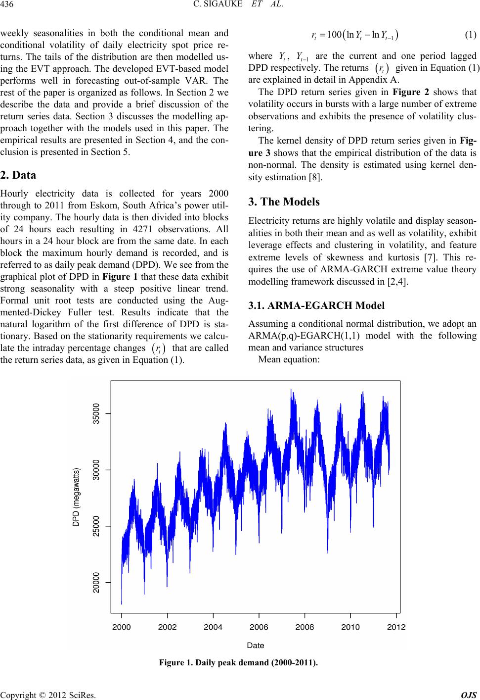. SIGAUKE ET AL.

436





100 lnln

ttt

rYY





Y Y

weekly seasonalities in both the conditional mean and

conditional volatility of daily electricity spot price re-

turns. The tails of the distribution are then modelled us-

ing the EVT approach. The developed EVT-based model

performs well in forecasting out-of-sample VAR. The

rest of the paper is organized as follows. In Section 2 we

describe the data and provide a brief discussion of the

return series data. Section 3 discusses the modelling ap-

proach together with the models used in this paper. The

empirical results are presented in Section 4, and the con-

clusion is presented in Section 5.

2. Data

Hourly electricity data is collected for years 2000

through to 2011 from Eskom, South Africa’s power util-

ity company. The hourly data is then divided into blocks

of 24 hours each resulting in 4271 observations. All

hours in a 24 hour block are from the same date. In each

block the maximum hourly demand is recorded, and is

referred to as daily peak demand (DPD). We see from the

graphical plot of DPD in Figure 1 that these data exh ibit

strong seasonality with a steep positive linear trend.

Formal unit root tests are conducted using the Aug-

mented-Dickey Fuller test. Results indicate that the

natural logarithm of the first difference of DPD is sta-

tionary. Based on the stationarity requirements we calcu-

late the intraday pe rcentage changes t that are called

the return series data, as given in Equation (1).

(1)

where t, 1t



are the current and one period lagged

DPD respectively. The returns t given in Equation (1)

are explained in detail in Appendix A.



The DPD return series given in Figure 2 shows that

volatility occurs in bursts with a large nu mber of extreme

observations and exhibits the presence of volatility clus-

tering.

The kernel density of DPD return series given in Fig-

ure 3 shows that the empirical distribution of the data is

non-normal. The density is estimated using kernel den-

sity estimation [8].

3. The Models

Electricity returns are highly volatile and display season-

alities in both their mean and as well as volatility, exhibit

leverage effects and clustering in volatility, and feature

extreme levels of skewness and kurtosis [7]. This re-

quires the use of ARMA-GARCH extreme value theory

modelling framework discussed in [2,4].

3.1. ARMA-EGARCH Model

Assuming a conditional normal d istribution, we adopt an

ARMA(p,q)-EGARCH(1,1) model with the following

mean and variance structures



rMean equation:

Figure 1. Daily peak demand (2000-2011).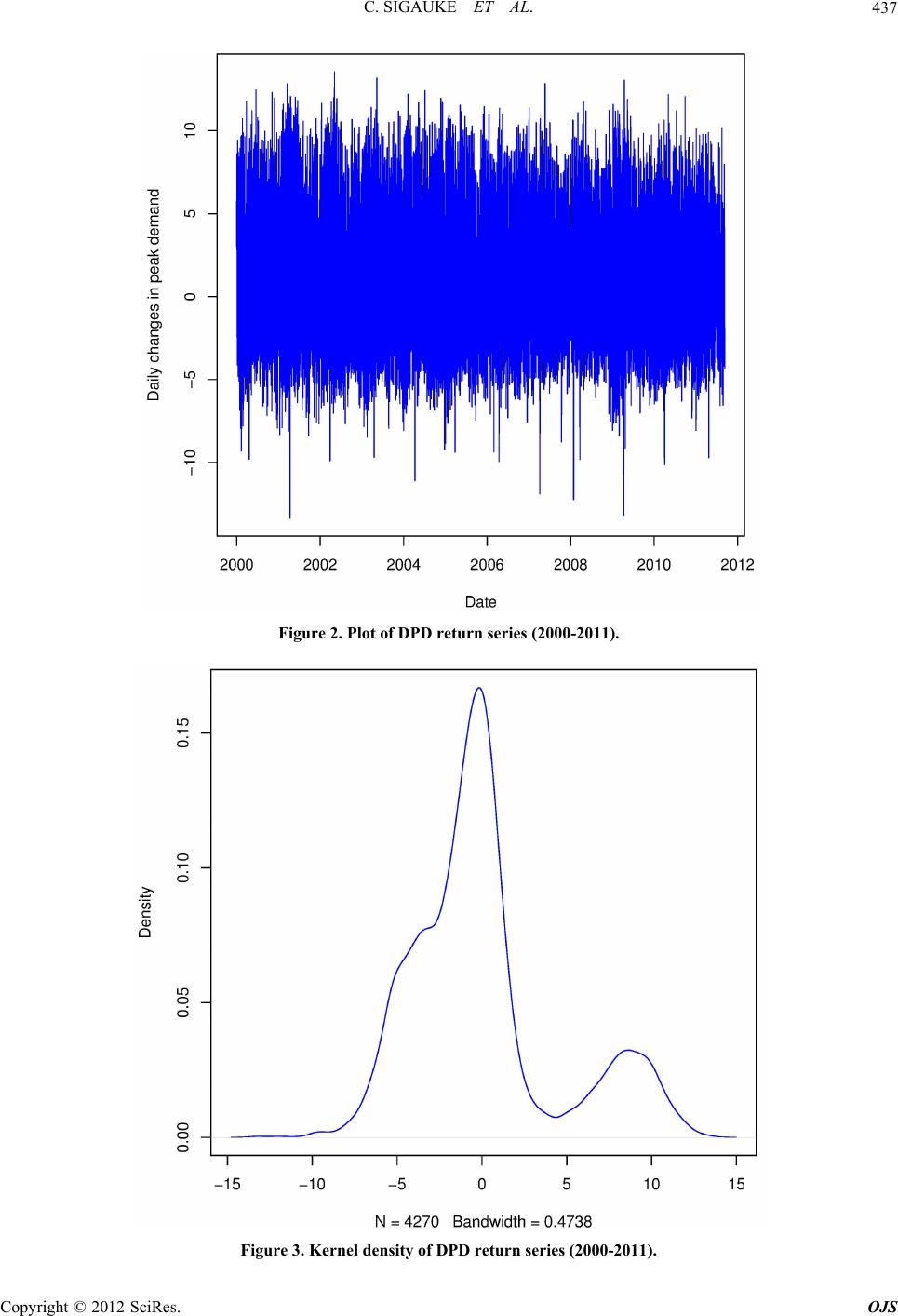

C. SIGAUKE ET AL. 437

Figure 2. Plot of DPD return series (2000-2011).

Figure 3. Kernel density of DPD return series (2000-2011).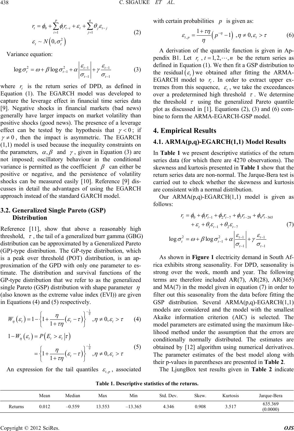

C. SIGAUKE ET AL.

CiRes. OJS

438

titjtj

with certain probabilities is given as:



~0,





















(2)

Variance equation:

log log



 









  (3)

where t is the return series of DPD, as defined in

Equation (1). The EGARCH model was developed to

capture the leverage effect in financial time series data

[9]. Negative shocks in financial markets (bad news)

generally have larger impacts on market volatility than

positive shocks (good news). The presence of a leverage

effect can be tested by the hypothesis that





; if





, then the impact is asymmetric. The EGARCH

(1,1) model is used because the inequality constraints on

the parameters,





and



, given in Equation (3) are

not imposed; oscillatory behaviour in the conditional

variance is permitted as the coefficient



can either be

positive or negative, and the persistence of volatility

shocks can be measured easily [10]. Reference [9] dis-

cusses in detail the advantages of using the EGARCH

approach instead of the standard GARCH model.

3.2. Generalized Single Pareto (GSP)

Distribution

Reference [11], show that above a reasonably high

threshold,



, the tail of a generalized burr gamma (GBG)

distribution can be approximated by a Generalized Pareto

(GP)-type distribution. The GP-type distribution, which

is a peak over threshold (POT) distribution, is an ap-

proximation of the GPD with only one parameter to es-

timate. The distribution and survival functions of the

GP-type distribution that we refer to as the generalized

single Pareto (GSP) distribution with shape parameter



(also known as the ex treme value index (EVI)) are giv en

in Equation s (4) and (5) respectively.

 



, 0,











 







 



 



(4)



ttt

WPE













 

,tp









 







(5)

An expression for the tail quantiles



, associated



,11 ,0,

tp t



 













, 1,2,,rt n

(6)

A derivation of the quantile function is given in Ap-

pendix B1. Let t



 be the return series as

defined in Equation (1). We then fit a GSP distribution to

the residual







we obtained after fitting the ARMA-

EGARCH model to t. In order to extract upper ex-

tremes from this sequence, t



, we take the exceedances

over a predetermined high threshold



. We determine

the threshold



using the generalized Pareto quantile

plot as discussed in [1]. Equations (2), (3) and (6) com-

bine to form the ARMA-EGARCH-GSP model.

4. Empirical Results

4.1. ARMA(p,q)-EGARCH(1,1) Model Results

In Table 1 we present descriptive statistics of the return

series data (for which there are 4270 observations). The

skewness and kurtosis presented in Table 1 show that the

return series data ar e non-normal. The Jarque-Bera test is

carried out to check whether the skewness and kurtosis

are consistent with a normal distribution.

Our ARMA(p,q)-EGARCH(1,1) model is given as

follows:

01 1273284365

1127

111

log log

ttttt

tt t

rrrrr

 

 



 



 









 

 

 

(7)

As shown in Figure 1 electricity demand in South Af-

rica exhibits strong seasonality. For DPD, seasonality is

strong over the week, month and year. The following

terms are therefore included AR(7), AR(28), AR(365)

and MA(7) in the model given in equation (7) in order to

filter out this seasonality from the data before fitting the

GSP distribution. Several ARMA(p,q)-EGARCH(1,1)

models are considered and the model with the smallest

Akaike information criterion (AIC) is selected. The

model parameters are estimated using the maximum like-

lihood method under the assumption that the errors are

conditionally normally distributed. The estimates are

obtained by [12] algorithm using numerical derivatives.

The parameter estimates of the best model along with

their p-values in parent heses are presented in Table 2.

The LjungBox test results given in Table 2 indicate

Table 1. Descriptive statistics of the returns.

Mean Median Max Min Std. Dev. Skew. Kurtosis Jarque-Bera

Returns 0.012 –0.559 13.553 –13.365 4.346 0.908 3.517 635.369

(0.0000)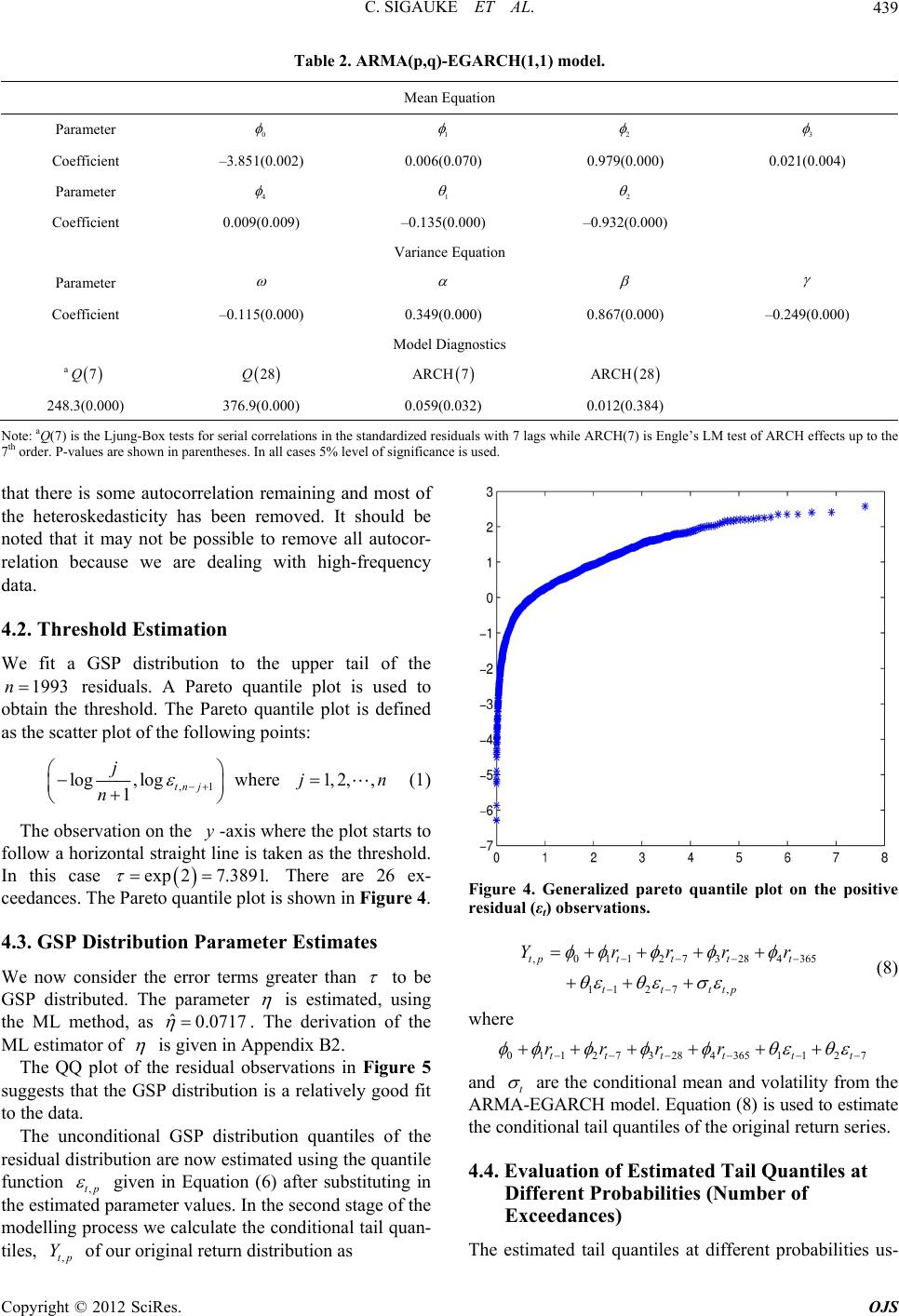

C. SIGAUKE ET AL. 439

Table 2. ARMA(p,q)-EGARCH(1,1) model.

Mean Equation

Parameter 0



Coefficient –3.851(0.002) 0.006(0.070) 0.979(0.000) 0.021(0.004)

Parameter 4





Coefficient 0.009(0.009) –0.135(0.000) –0.932(0.000)

Variance Equation

Parameter









Coefficient –0.115(0.000) 0.349(0.000) 0.867(0.000) –0.249(0.000)

Model Diagnostics



28Q





ARCH7





ARCH28

248.3(0.000) 376.9(0.000) 0.059(0.032) 0.012(0.384)

Note: aQ(7) is the Ljung-Box tests for serial correlations in the standardized residuals with 7 lags while ARCH(7) is Engle’s LM test of ARCH effects up to the

7th order. P-values are shown in parentheses. I n all cases 5% level of significance is used.

that there is some autocorrelation remaining and most of

the heteroskedasticity has been removed. It should be

noted that it may not be possible to remove all autocor-

relation because we are dealing with high-frequency

data.

4.2. Threshold Estimation

We fit a GSP distribution to the upper tail of the

residuals. A Pareto quantile plot is used to

obtain the threshold. The Pareto quantile plot is defined

as the scatter plot of the following points:

1993n

log ,logwhere

1tn j











1,2, ,

jjn







exp 27.3891.





(1)

The observation on the -axis where the plot starts to

follow a horizontal straight line is taken as the threshold.

In this case There are 26 ex-

ceedances. The Pareto quantile plot is shown in Figure 4.

4.3. GSP Distribution Parameter Estimates

We now consider the error terms greater than



to be

GSP distributed. The parameter



is estimated, using

the ML method, as ˆ0.0717



. The derivation of the

ML estimator of



is given in Appendix B2.

The QQ plot of the residual observations in Figure 5

suggests that the GSP distribution is a relatively good fit

to the data.

The unconditional GSP distribution quantiles of the

residual distribution are now estimated using the quantile

function ,tp

Figure 4. Generalized pareto quantile plot on the positive

residual (εt) observations.

,011273 284 365

112 7,

tpt ttt

ttttp

Yrrrr

 

 

 



 

 

01127328436511 27ttttt t

rrr r

(8)

where



given in Equation (6) after substituting in

the estimated parameter values. In the second stage of th e

modelling process we calculate the co nditional tail quan-

tiles, of our origin al return distribution as

,tp

 

 







 

and t



are the conditional mean and volatility from the

ARMA-EGARCH model. Equation (8) is used to estimate

the conditional tail quantiles of the original return series.

4.4. Evaluation of Estimated Tail Quantiles at

Different Probabilities (Number of

Exceedances)

The estimated tail quantiles at different probabilities us-

C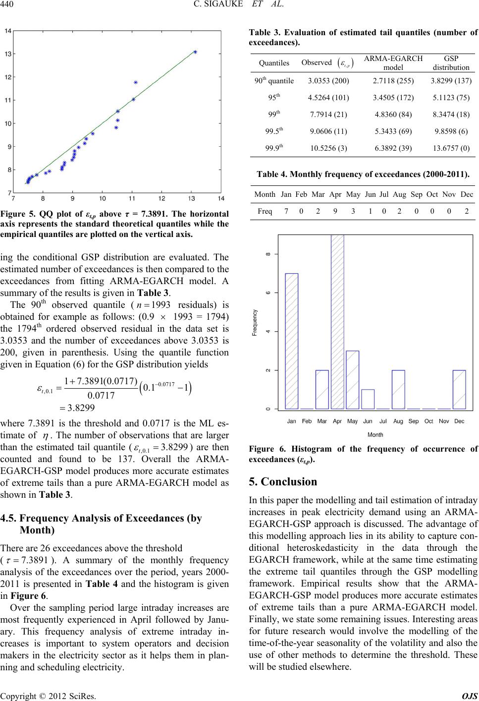. SIGAUKE ET AL.

440

Figure 5. QQ plot of εt,p above τ = 7.3891. The horizontal

axis represents the standard theoretical quantiles while the

empirical quantiles are plotted on the vertical axis.

ing the conditional GSP distribution are evaluated. The

estimated number of exceedances is then compared to the

exceedances from fitting ARMA-EGARCH model. A

summary of the results is given in Table 3.

The 90th observed quantile ( residuals) is

obtained for example as follows: (0.9 1993 = 1794)

the 1794th ordered observed residual in the data set is

3.0353 and the number of exceedances above 3.0353 is

200, given in parenthesis. Using the quantile function

given in Equation (6) for the GSP distribution yields

1993n





0.0717

0.1 1





,0.1 1 7.3891(0.0717)

0.0717

3.8299







where 7.3891 is the threshold and 0.0717 is the ML es-

timate of



. The number of observations that are larger

than the estimated tail quantile (,0.1t3.8299





7.3891

) are then

counted and found to be 137. Overall the ARMA-

EGARCH-GSP model produces more accurate estimates

of extreme tails than a pure ARMA-EGARCH model as

shown in Table 3.

4.5. Frequency Analysis of Exceedances (by

Month)

There are 26 exceedances above the threshold

(



). A summary of the monthly frequency

analysis of the exceedances over the period, years 2000-

2011 is presented in Table 4 and the histogram is given

in Figure 6.

Over the sampling period large intraday increases are

most frequently experienced in April followed by Janu-

ary. This frequency analysis of extreme intraday in-

creases is important to system operators and decision

makers in the electricity sector as it helps them in plan-

ning and scheduling electricity.

Table 3. Evaluation of estimated tail quantiles (number of

exceedances).





Quantiles Observed ,tp



ARMA-EGARCH

model GSP

distribution

90th quantile3.0353 (200) 2.7118 (255) 3.8299 (137)

95th 4.5264 (101) 3.4505 (172) 5.1123 (75)

99th 7.7914 (21) 4.8360 (84) 8.3474 (18)

99.5th 9.0606 (11) 5.3433 (69) 9.8598 (6)

99.9th 10.5256 (3) 6.3892 (39) 13.6757 (0)

Table 4. Monthly frequency of exceedances (2000-2011).

MonthJanFebMarAprMay Jun Jul Aug Sep OctNovDec

Freq702931 0 2 0 002

Figure 6. Histogram of the frequency of occurrence of

exceedances (εt,p).

5. Conclusion

In this paper the modelling and tail estimation of intrad ay

increases in peak electricity demand using an ARMA-

EGARCH-GSP approach is discussed. The advantage of

this modelling approach lies in its ability to capture con-

ditional heteroskedasticity in the data through the

EGARCH framework, while at the same time estimating

the extreme tail quantiles through the GSP modelling

framework. Empirical results show that the ARMA-

EGARCH-GSP model produces more accurate estimates

of extreme tails than a pure ARMA-EGARCH model.

Finally, we state some remaining issues. Interesting areas

for future research would involve the modelling of the

time-of-the-year seasonality of the volatility and also the

use of other methods to determine the threshold. These

will be studied elsewhere.

C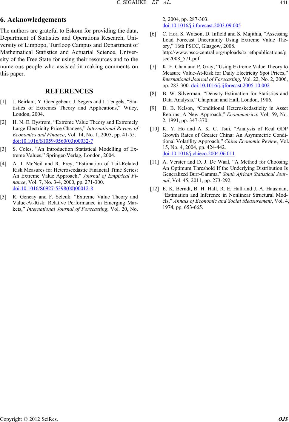. SIGAUKE ET AL.

441

6. Acknowledgements

The authors are grateful to Eskom for providing the data,

Department of Statistics and Operations Research, Uni-

versity of Limpopo, Turfloop Campus and Department of

Mathematical Statistics and Actuarial Science, Univer-

sity of the Free State for using their resources and to the

numerous people who assisted in making comments on

this paper.

REFERENCES

[1] J. Beirlant, Y. Goedgebeur, J. Segers and J. Teugels, “Sta-

tistics of Extremes Theory and Applications,” Wiley,

London, 2004.

[2] H. N. E. Bystrom, “Extreme Value Theory and Extremely

Large Electricity Price Changes,” International Review of

Economics and Finance, Vol. 14, No. 1, 2005, pp. 41-55.

doi:10.1016/S1059-0560(03)00032-7

[3] S. Coles, “An Introduction Statistical Modelling of Ex-

treme Values,” Springer-Verlag, London, 2004.

[4] A. J. McNeil and R. Frey, “Estimation of Tail-Related

Risk Measures for Heteroscedastic Financial Time Series:

An Extreme Value Approach,” Journal of Empirical Fi-

nance, Vol. 7, No. 3-4, 2000, pp. 271-300.

doi:10.1016/S0927-5398(00)00012-8

[5] R. Gencay and F. Selcuk. “Extreme Value Theory and

Value-At-Risk: Relative Performance in Emerging Mar-

kets,” International Journal of Forecasting, Vol. 20, No.

2, 2004, pp. 287-303.

doi:10.1016/j.ijforecast.2003.09.005

[6] C. Hor, S. Watson, D. Infield and S. Majithia, “Assessing

Load Forecast Uncertainty Using Extreme Value The-

ory,” 16th PSCC, Glasgow, 2008.

http://www.pscc-central.org/uploads/tx_ethpublications/p

scc2008_571.pdf

[7] K. F. Chan and P. Gray, “Using Extreme Value Theory to

Measure Value-At-Risk for Daily Electricity Spot Prices,”

International Journal of Foreca sting, Vol. 22, No. 2, 2006,

pp. 283-300. doi:10.1016/j.ijforecast.2005.10.002

[8] B. W. Silverman, “Density Estimation for Statistics and

Data Analysis,” Chapman and Hall, London, 1986.

[9] D. B. Nelson, “Conditional Heteroskedasticity in Asset

Returns: A New Approach,” Econometrica, Vol. 59, No.

2, 1991, pp. 347-370.

[10] K. Y. Ho and A. K. C. Tsui, “Analysis of Real GDP

Growth Rates of Greater China: An Asymmetric Condi-

tional Volatility Approach,” China Economic Review, Vol.

15, No. 4, 2004, pp. 424-442.

doi:10.1016/j.chieco.2004.06.011

[11] A. Verster and D. J. De Waal, “A Method for Choosing

An Optimum Threshold If the Underlying Distribution Is

Generalized Burr-Gamma,” South African Statistical J our-

nal, Vol. 45, 2011, pp. 273-292.

[12] E. K. Berndt, B. H. Hall, R. E. Hall and J. A. Hausman,

“Estimation and Inference in Nonlinear Structural Mod-

els,” Annals of Economic and Social Measurement, Vol. 4,

1974, pp. 653-665.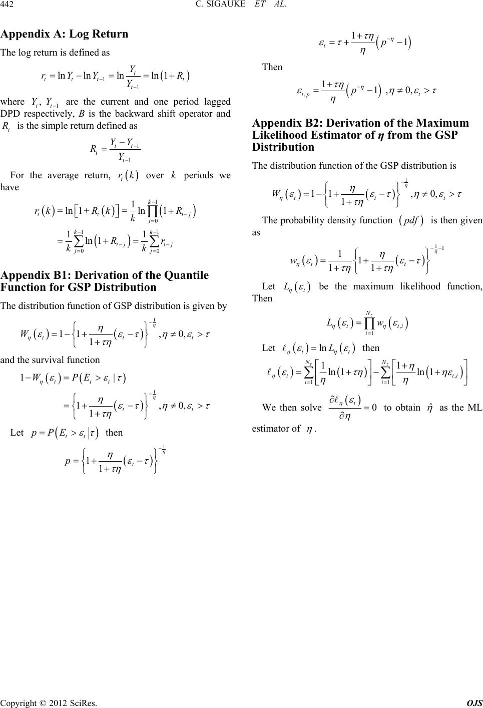

C. SIGAUKE ET AL.

442

Appendix A: Log Return

The log return is defined as



ln 1t



lnlnln t

ttt t

rYY Y



 

where 1tt are the current and one period lagged

DPD respectively, B is the backward shift operator and

is the simple return defined as





For the average return,





rk k

t over periods we

have

 



















ln 1ln

ln 1

rkRk k

 





Appendix B1: Derivation of the Quantile

Function for GSP Distribution

The distributio n function of GSP dist ri b ut ion is gi ven by

 



, 0,











 







 



 



and the survival function

 



ttt

WPE













 









 







Let



pPE





 then





























 







Then



,11 ,0,

tp t



 















Appendix B2: Derivation of the Maximum

Likelihood Estimator of η from the GSP

Distribution

The distributio n function of the GSP dist ribution is



11, 0,

ttt



 











 









pdf



The probability dens ity function is then given







 



















Let



be the maximum likelihood function,

Then



tti























Let







then



ln 1ln 1

tti





 







 



 



 



 









We then solve 0













ˆ

to obtain



as the ML

estimator of

