

Paper Menu >>
Journal Menu >>
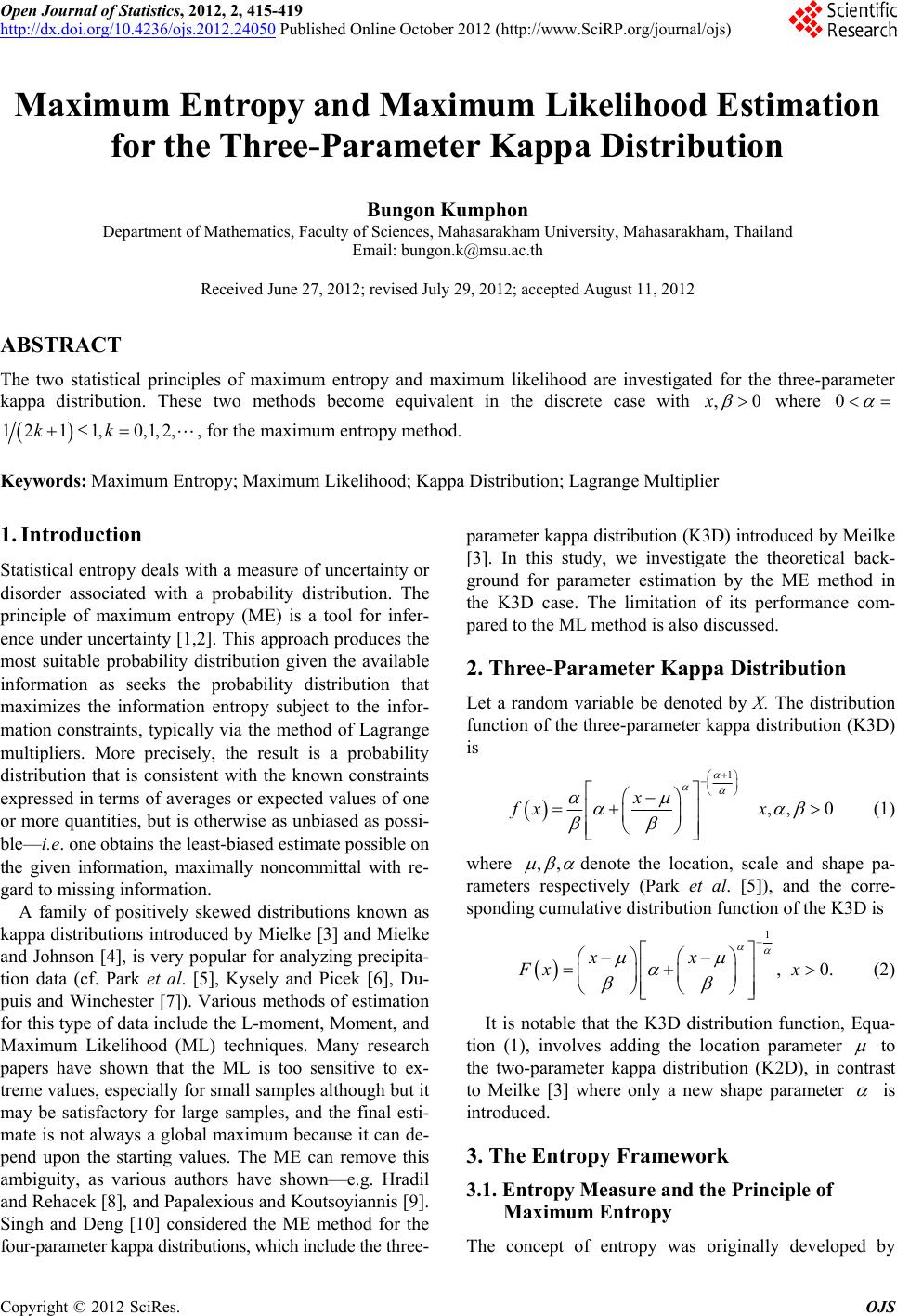 Open Journal of Statistics, 2012, 2, 415-419 http://dx.doi.org/10.4236/ojs.2012.24050 Published Online October 2012 (http://www.SciRP.org/journal/ojs) Maximum Entropy and Maximum Likelihood Estimation for the Three-Parameter Kappa Distribution Bungon Kumphon Department of Mathematics, Faculty of Sciences, Mahasarakham University, Mahasarakham, Thailand Email: [email protected] Received June 27, 2012; revised July 29, 2012; accepted August 11, 2012 ABSTRACT The two statistical principles of maximum entropy and maximum likelihood are investigated for the three-parameter kappa distribution. These two methods become equivalent in the discrete case with ,0x where 0 1211,0,1,2,kk , for the maximum entropy method. Keywords: Maximum Entropy; Maximum Likelihood; Kapp a Distribution; Lagran ge Multiplier 1. Introduction Statistical entropy deals with a measure of uncertainty or disorder associated with a probability distribution. The principle of maximum entropy (ME) is a tool for infer- ence under uncertainty [1,2]. This approach produces the most suitable probability distribution given the available information as seeks the probability distribution that maximizes the information entropy subject to the infor- mation constraints, typically via the method of Lagrange multipliers. More precisely, the result is a probability distribution that is consistent with the known constraints expressed in terms of averages or expected values of one or more quantities, but is otherwise as unbiased as possi- ble—i.e. one obtains the least-biased estimate possible on the given information, maximally noncommittal with re- gard to missing information. A family of positively skewed distributions known as kappa distributions introduced by Mielke [3] and Mielke and Johnson [4], is very popular for analyzing precipita- tion data (cf. Park et al. [5], Kysely and Picek [6], Du- puis and Winchester [7]). Various methods of estimation for this type of data include the L-moment, Moment, and Maximum Likelihood (ML) techniques. Many research papers have shown that the ML is too sensitive to ex- treme values, especially for small samples although but it may be satisfactory for large samples, and the final esti- mate is not always a global maximum because it can de- pend upon the starting values. The ME can remove this ambiguity, as various authors have shown—e.g. Hradil and Rehacek [8], and Papalexious and Koutsoyiannis [9]. Singh and Deng [10] considered the ME method for the four-parameter kappa distributions, which include the three- parameter kappa distribution (K3D) introduced by Mei lke [3]. In this study, we investigate the theoretical back- ground for parameter estimation by the ME method in the K3D case. The limitation of its performance com- pared to the ML method is also discussed. 2. Three-Parameter Kappa Distribution Let a random variable be denoted by X. The distribution function of the three-parameter kappa distribution (K3D) is 1 ,, 0 x fx x ,, (1) where denote the location, scale and shape pa- rameters respectively (Park et al. [5]), and the corre- sponding cumulative d istribution function of the K3D is 1 ,0. xx Fx x (2) It is notable that the K3D distribution function, Equa- tion (1), involves adding the location parameter to the two-parameter kappa distribution (K2D), in contrast to Meilke [3] where only a new shape parameter is introduced. 3. The Entropy Framework 3.1. Entropy Measure and the Principle of Maximum Entropy The concept of entropy was originally developed by C opyright © 2012 SciRes. OJS 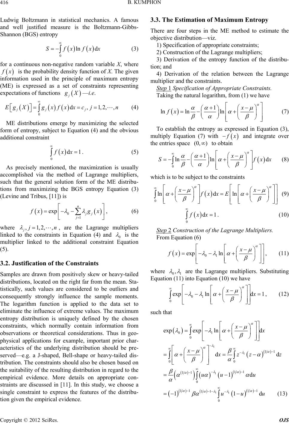 B. KUMPHON 416 Ludwig Boltzmann in statistical mechanics. A famous and well justified measure is the Boltzmann-Gibbs- Shannon (BGS) entropy ln dxfxx 0 Sf (3) for a continuous non-negative random variable X, where f x is the probability density fu nction of X. The given information used in the principle of maximum entropy (ME) is expressed as a set of constraints representing expectations of funct i o ns j g X 1,2,, j j n 0 d1fx x —i.e. 0 d, jj EgXg xfx x c (4) ME distributions emerge by maximizing the selected form of entropy, subject to Equation (4) and the obvious additional con strain t 1 n jj j . (5) As precisely mentioned, the maximization is usually accomplished via the method of Lagrange multipliers, such that the general solution form of the ME distribu- tions from maximizing the BGS entropy Equation (3) (Levine and Tribus, [11]) is 0 exp f x gx ,1,2,,jn , (6) where j , are the Lagrange multipliers linked to the constraints in Equation (4) and 0 is the multiplier linked to the additional constraint Equation (5). 3.2. Justification of the Constraints Samples are drawn from positively skew or heavy-tailed distributions, located on the right far from the mean. Sta- tistically, such values are considered to be outliers and consequently strongly influence the sample moments. The logarithm function is applied to the data set to eliminate the influence of extreme values. The maximum entropy distribution is uniquely defined by the chosen constraints, which normally contain information from observations or theoretical considerations. Thus in geo- physical applications for example, important prior char- acteristics of the underlying distribution should be pre- served—e.g. a J-shaped, Bell-shape or heavy-tailed dis- tribution. The constraints should also be chosen based on the suitability of the resulting distribution in regard to the empirical evidence. More details on appropriate con- straints are discussed in [11]. In this study, we choose a single constraint to express the features of the distribu- tion given the empirical evidence. 3.3. The Estimation of Maximum Entropy There are four steps in the ME method to estimate the objective distribution—viz. 1) Specification of appropriate constraints; 2) Construction of the Lagrange multipliers; 3) Derivation of the entropy function of the distribu- tion; and 4) Derivation of the relation between the Lagrange multiplier and the constraints. Step 1 Specification of Appropriate Constraints. Taking the natural logarithm, from (1) we have 1 lnlnln x fx (7) To establish the entropy as expressed in Equation (3), multiply Equation (7) with f x (0, ) and integrate over the entries space to obtain 0 1 ln lnd x Sfxx (8) which is to be subject to the constraints 0 lnd ln xx fx xE 0 d1fx x (9) . (10) Step 2 Construction of the Lag r ange Multipliers. From Equation (6) 01 explnx fx , (11) , where 01 are the Lagrange multipliers. Substituting Equation (11) into Equat i o n ( 10) we have 01 0 explnd 1 xx , (12) such that 1 1 1 11 01 0 11 00 11 11 0 11 11 11 0 expexp lnd dd 1d 11d (13) xx x x zz z uu u uu u Copyright © 2012 SciRes. OJS 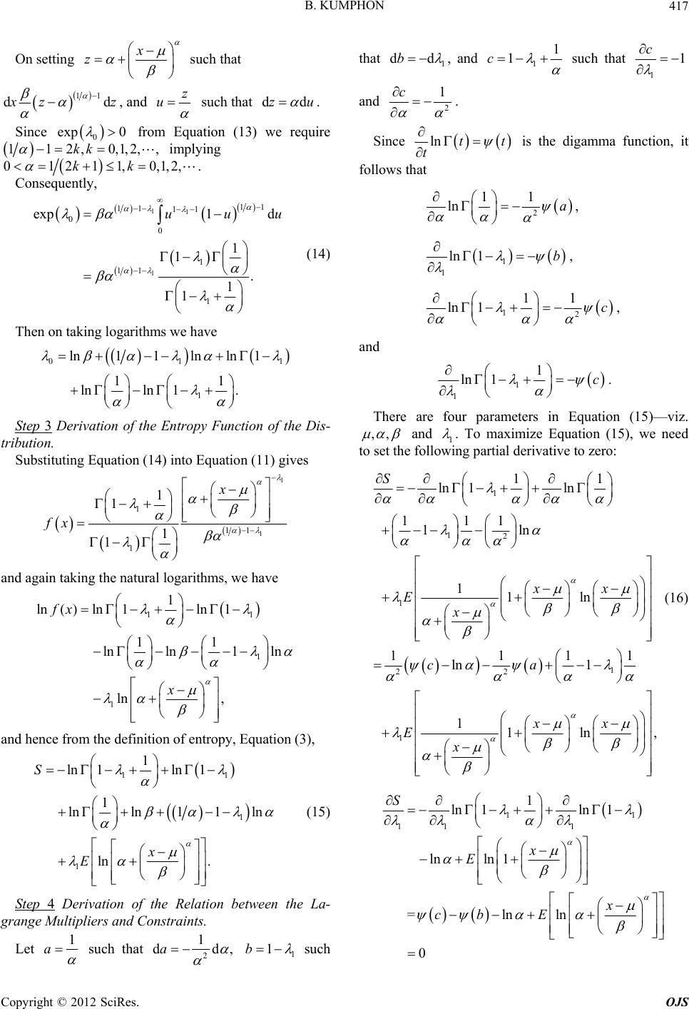 B. KUMPHON 417 On setting x z such that 11 dd x zz , and z u zu such that dd . Since from Equation (13) we require 0 exp 0 112, 0,1,2, ,kk implying 01 211 , 0,1,2,kk. Consequently, 11 1 11 11 00 1 11 1 exp 1 1 1 11 d 1 . 1 uuu (14) Then on taking logarithms we have 01 1 ln1 1 ln lnln 1 1 ln 1 11 . Step 3 Derivation of the Entropy Function of the Dis- tribution. Substituting Equation (14) into Equation (11) gives 1 1 11 x 1 1 1 1 1 1 fx and again taking the natural logarithms, we have 11 1 1 1 ln , 1 1 ln( )ln1ln 11 ln ln ln fx x and hence from the definition of entropy, Equation (3), 11 1 1 1 ln . 1 1 ln 1ln 1 lnln 1 ln S x E (15) Step 4 Derivation of the Relation between the La- grange Multipliers and Constraints. Let 1 a such that 2 dda1, 1 1b 1 ddb such that , and 11 1c such that 1 1 c and 2 1c . Since ln tt t is the digamma function, it follows that 2 11 ln a , 1 1 ln 1b , 12 11 ln 1c , and 1 1 1 ln 1c ,, . There are four parameters in Equation (15)—viz. and 1 . To maximize Equation (15), we need to set the following partial d erivative to zero: 1 12 1 1 22 1 11 ln 1ln 111 1ln 11ln 1111 ln 1 11ln S xx Ex ca xx Ex (16) , 11 11 1 1 ln1ln 1 lnln 1 =lnln 0 S x E x cb E Copyright © 2012 SciRes. OJS 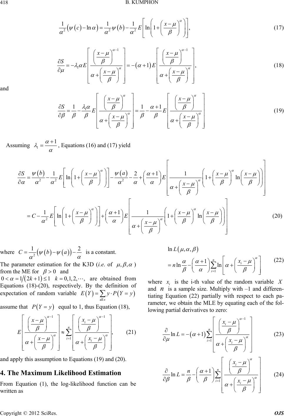 B. KUMPHON OJS 418 222 111 lnln 1cbE , x (17) 11 1, xx E xx 1 SE (18) and 1 11SE 1 xx E xx (19) Copyright © 2012 SciRes. Assuming 11 , Equations (16) and (17) yield 22 2 2 1211 ln 11ln 111 ln 11 ba Sx x EE x xx CEE x x ln x (20) where 2 Cb 12 a ,, is a constant. The parameter estimation for the K3D (i.e. of 0) from the ME for and 012110,1,kk 2,, are obtained from Equations (18)-(20), respectively. By the definition of expectation of random variable x EYyPY y all assume that PY y equal to 1, thus Equation (18), 11 , i i x x 1 n i x Ex (21) and apply this assumption to Equations (19) and (20). 4. The Maximum Likelihood Estimation From Equation (1), the log-likelihood function can be written as 1 ln, , 1 ln ln ni i L x n (22) where i x is the i-th value of the random variable X and is a sample size. Multiply with –1 and differen- tiating Equation (22) partially with respect to each pa- rameter, we obtain the MLE by equating each of the fol- lowing partial derivatives to zero: n 1 1 ln 1 i n ii x Lx (23) 1 1 ln i n ii x n Lx (24) 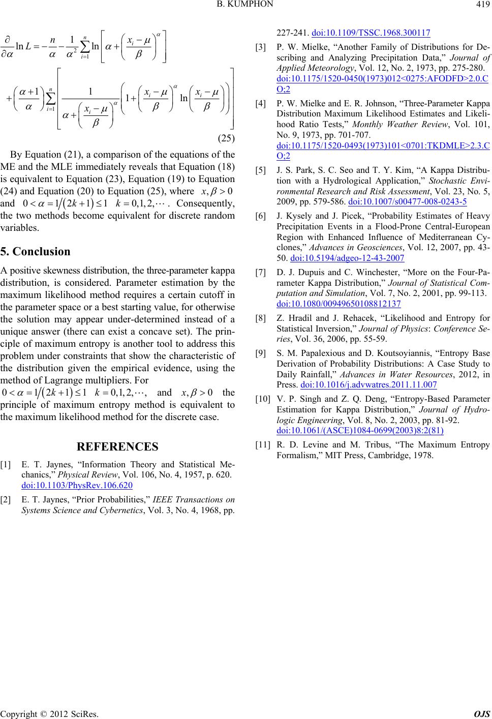 B. KUMPHON 419 21 1 1 ln ln 11 1l ni i n ii x n L x n ii xx ,0x (25) By Equation (21), a comparison of the equations of the ME and the MLE immediately reveals that Equation (18) is equivalent to Equation (23), Equation (19) to Equation (24) and Equation (20) to Equation (25), where and 01211kk 0,1,2,. Consequently, the two methods become equivalent for discrete random variables. 5. Conclusion A positive skewness distribution, the three-parameter ka p pa distribution, is considered. Parameter estimation by the maximum likelihood method requires a certain cutoff in the parameter space or a best starting value, for otherwise the solution may appear under-determined instead of a unique answer (there can exist a concave set). The prin- ciple of maximum entropy is another tool to address this problem under constraints that show the characteristic of the distribution given the empirical evidence, using the method of Lagrange multipliers. For 01211kk ,0x0,1,2,, and the principle of maximum entropy method is equivalent to the maximum likelihood method for the discrete case. REFERENCES [1] E. T. Jaynes, “Information Theory and Statistical Me- chanics,” Physical Review, Vol. 106, No. 4, 1957, p. 620. doi:10.1103/PhysRev.106.620 [2] E. T. Jaynes, “Prior Probabilities,” IEEE Transactions on Systems Science and Cybernetics, Vol. 3, No. 4, 1968, pp. 227-241. doi:10.1109/TSSC.1968.300117 [3] P. W. Mielke, “Another Family of Distributions for De- scribing and Analyzing Precipitation Data,” Journal of Applied Meteorology, Vol. 12, No. 2, 1973, pp. 275-280. doi:10.1175/1520-0450(1973)012<0275:AFODFD>2.0.C O;2 [4] P. W. Mielke and E. R. Johnson, “Three-Parameter Kap pa Distribution Maximum Likelihood Estimates and Likeli- hood Ratio Tests,” Monthly Weather Review, Vol. 101, No. 9, 1973, pp. 701-707. doi:10.1175/1520-0493(1973)101<0701:TKDMLE>2.3.C O;2 [5] J. S. Park, S. C. Seo and T. Y. Kim, “A Kappa Distribu- tion with a Hydrological Application,” Stochastic Envi- ronmental Research and Risk Assessment, Vol. 23, No. 5, 2009, pp. 579-586. doi:10.1007/s00477-008-0243-5 [6] J. Kysely and J. Picek, “Probability Estimates of Heavy Precipitation Events in a Flood-Prone Central-European Region with Enhanced Influence of Mediterranean Cy- clones,” Advances in Geosciences, Vol. 12, 2007, pp. 43- 50. doi:10.5194/adgeo-12-43-2007 [7] D. J. Dupuis and C. Winchester, “More on the Four-Pa- rameter Kappa Distribution,” Journal of Statistical Com- putation and Simulation, Vol. 7, No. 2, 2001, pp. 99-113. doi:10.1080/00949650108812137 [8] Z. Hradil and J. Rehacek, “Likelihood and Entropy for Statistical Inversion,” Journal of Physics: Conference Se- ries, Vol. 36, 2006, pp. 55-59. [9] S. M. Papalexious and D. Koutsoyiannis, “Entropy Base Derivation of Probability Distributions: A Case Study to Daily Rainfall,” Advances in Water Resources, 2012, in Press. doi:10.1016/j.advwatres.2011.11.007 [10] V. P. Singh and Z. Q. Deng, “Entropy-Based Parameter Estimation for Kappa Distribution,” Journal of Hydro- logic Engineering, Vol. 8, No. 2, 2003, pp. 81-92. doi:10.1061/(ASCE)1084-0699(2003)8:2(81) [11] R. D. Levine and M. Tribus, “The Maximum Entropy Formalism,” MIT Press, Cambridge, 1978. Copyright © 2012 SciRes. OJS |