Artificial Neural Networks for Event Based Rainfall-Runoff Modeling

doi:10.4236/jwarp.2012.410105

Paper Menu >>

Journal Menu >>

Journal of Water Resource and Protection, 2012, 4, 891-897

http://dx.doi.org/10.4236/jwarp.2012.410105 Published Online October 2012 (http://www.SciRP.org/journal/jwarp)

Artificial Neural Networks for Event Based

Rainfall-Runoff Modeling

Archana Sarkar, Rakesh Kumar

National Institute of Hydrology, Roorkee, India

Email: [email protected]

Received March 11, 2012; revised May 19, 2012; accepted August 12, 2012

ABSTRACT

The Artificial Neural Network (ANN) approach has been successfully used in many hydrological studies especially the

rainfall-runoff modeling using continuous data. The present study examines its applicability to model the event-based

rainfall-runoff process. A case study has been done for Ajay river basin to develop event-based rainfall-runoff model

for the basin to simulate the hourly runoff at Sarath gauging site. The results demonstrate that ANN mod els are able to

provide a good r epresentation of an even t-based rainfa ll-runo ff process. The two impor tant pa rameters, when predictin g

a flood hydrograph, are the magnitude of the peak discharge and the time to peak discharge. The developed ANN mod-

els have been able to predict this information with great accuracy. This shows that ANNs can be very efficient in mod-

eling an even t-based rainfall-runoff process for determining the peak discharge and time to the peak discharge very ac-

curately. This is important in water resources design and management applications, where peak discharge and time to

peak discharge are important input variables.

Keywords: Artificial Neural Networks (ANNs); Event Based Rainfall-Runoff Process; Error Back Propagation; Neural

Power

1. Introduction

Rainfall-runoff is important in activities such as flood

control and management, design of hydraulic structures

in a watershed, and likewise. Historically, researchers

have relied on conventional techniques, either determi-

nistic models, which consider the physics of the under-

lying process, or systems theoretic/black-box models,

which do not. Determi ni s t i c m odels of varying degrees of

complexity have been employed in the past for the rain-

fall runoff process with varying degrees of success. The

rainfall runoff is a complex, dynamic, and non-linear

process, which is affected by many and often interrelated,

physical factors. The influence of these factors and many

of their combinations in generating runoff is an ex-

tremely complex physical process, and is not clearly un-

derstood [1]. Moreover, many of the deterministic rain-

fall-runoff models need a large amount of data for cali-

bration and validation purposes, and are computationally

expensive. As a result, the use of deterministic models of

the rainfall-runoff process is viewed rather skeptically by

researchers and consequently has not become very popu-

lar [2].

Artificial Neural Networks (ANNs) have been pro-

posed as efficient tools for and prediction in hydrology,

as black-box models. ANNs are supposed to posses the

capability to reprodu ce the unknown relationsh ip ex isting

between a set of input variables (e.g., rainfall) of the sys-

tem and one or more output variables (e .g., runoff) [3]. In

recent years ANNs have shown exceptional performance

as regression tools, especially when used for pattern rec-

ognition and function estimation. They are highly non-

linear, and can capture complex interactions among the

input variables in a system without any prior knowledge

about the nature of these interactions [4]. The main ad-

vantage of ANNs is that one does not have to explicitly

assume a model form, which is a prerequisite in conven-

tional approaches. Ind eed, in ANNs the data poin ts them-

selves generate a relationship of possibly complicated or

orthodox shape. In comparison to the conventio nal meth-

ods, ANNs tolerate imprecise or incomplete data, ap-

proximate results, and are less vulnerable to outliers [5].

They are highly parallel, i.e., their numerous independent

operations can be executed simultaneously. These char-

acteristics render ANNs to be very suitable tools for han-

dling various hydrological problems. Although applica-

tion of ANN approach for rainfall-runoff process is re-

cent, it has already produced very encouraging results.

Among various hydrological problems, rainfall-runoff

has perhaps received the maximum attention from ANN

researchers. In an earlier study, Halff et al. [6] design ed a

three-layer feedforward ANN using the observed rainfall

A. SARKAR, R. KUMAR

892

hyetographs as inputs and hydrographs recorded by the

US Geological Survey (USGS) at Bellvue, Washington,

as outputs. This study opened up several possibilities for

rainfall-runoff application using neural networks. Hjelm-

felt and Wang [7] developed a neural network based on

the unit hydrograph theory for the Goodwater Creek wa-

tershed in central Missouri. In an application using two

neural networks, Zhu et al. [8] predicted upper and lower

bounds on the flood hydrograph in Butter Creek, New

York. Smith [9] used a back-propagation ANN model to

predict the peak discharge and the time to peak resulting

from a single rainfall pattern. Carriere et al. [10] de-

signed and developed a Virtual Runoff Hydrograph Sys-

tem (VROHS) based on ANN to generate runoff hydro-

graph. Lange [11] introduced a method which generates a

spe cial hydrograph (comparable with the unit hydrograph)

by using an ANN. Anmala et al. [12] utilized ANNs for

runoff predictions in three watersheds in Kansas. The

authors found that a direct use of feed forward ANNs

without time delayed input does not prov ide a significant

improvement over other regression techniques. Sudheer

et al. [13] worked on a data driven algorithm for con-

structing Artificial Neural Network Rainfall-Runoff

Models. Quebec. Chibanga et al. [14] modeled the de-

rived flow series (by simple reservoir routing) and the

time series of historic flow measured at the Kafue Hook

Bridge (KHB), Kafue River basin in Vietnam, separately

using ANNs. Chiang et al. [15] presented a system com-

parison of two basic types of neural networks, static and

dynamic in their study. Jy S. Wu et al. [16] demonstrated

the application of ANNs for watershed-runoff and

stream-flow forecasts. Sarkar et al. [17] developed back

propagation ANN runof f models to simulate and forecast

daily runoff for a part of the Satluj river basin of India.

Kisi [18] presented a comparison of different artificial

neural network algorithms for short term daily stream-

flow forecasting. Kalteh [19] developed rainfall-runoff

model using ANN and described different approaches

including Neural Interpretation Diagram, Garson’s algo-

rithm, and randomization approach to understand the

relationship learned by the ANN model. Modarres [20]

carried out a comprehensive multicriteria validation test

for rainfall-runoff by artificial neural networks with 17

global statistics and 3 additional non-parametric tests

through a case study of the Plasjan Basin in the western

region of the Zayandehrud watershed, Iran. Dorum et al.

[21] tried to set up rainfall-runoff relationship by using

ANN and Adaptive Neuro Fuzzy Interference Systems

(ANFIS) models at Flow Observation Stations on seven

sites in Susurluk Basin.

A rainfall-runoff model can be one of two types—an

event based rainfall-runoff model or a continuous rain-

fall-runoff model. Application of ANN approach for the

continuous rainfall-runoff process is numerous but that of

the event based process are limited. The present study

focuses on the of an event-based rainfall-runoff process.

Such ANN models are very useful in real time flood

forecasting.

2. Methodology

An ANN is a computing system made up of a highly in-

terconnected set of simple information processing ele-

ments, analogous to a neuron, called units. The neuron

collects inputs from both a single and multiple sources

and produces output in accordance with a predetermined

non-linear function. An ANN model is created by inter-

connection of many of the neurons in a known configu-

ration. The primary elements characterising the neural

network are the distributed representation of information,

local operations and non-linear processing. The theory of

ANN has been described in many books such as Haykin

[5] and Yegnanar ayana [22].

The main principle of neural computing is the decom-

position of the input-output relationship into series of

linearly separable steps using hidden layers [5]. Gener-

ally there are four distinct steps in developing an ANN-

based solution. The first step is the data transformation or

scaling. The second step is the network architecture defi-

nition, where the number of hidden layers, the number of

neurons in each layer, and the connectivity between the

neurons are set. In the third step, a learning algorithm is

used to train the network to respond correctly to a given

set of inputs. Lastly, comes the validation step in which

the performance of the trained ANN model is tested

through some selected statistical criteria.

Large variation in the input data can slow down or

even prevent the training of the network. To overcome

this potential problem, the data are usually scaled using

linear, logarithmic, or normal transformations. It is also

important that the absolute input values are scaled to

avoid asymptotic issues [5]. In the present study, the in-

put data for a variable x were standardised through the

ANN software, Neural Power [23].

There are three basic layers or levels of data process-

ing units viz., the input layer, the hidden layer and the

output layer. Each of these layers consists of processing

units called nodes of the neural network. The number of

input nodes, output nodes and the nodes in the hidden

layer depend upon the problem being studied. If the

number of nodes in the hidden layer is small, the network

may not have sufficient degrees of freedom to learn the

process correctly. If the number is too high, the training

will take a long time and the network may sometimes

over-fit the data [24].

The process of determining ANN weights is called

training, which forms the interconnection between neu-

rons. The ANNs are trained with a training set of input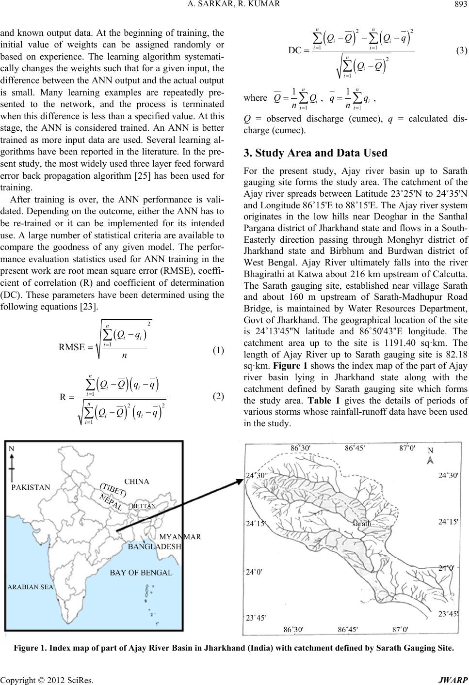

A. SARKAR, R. KUMAR

893





and known output data. At the beginning of training, the

initial value of weights can be assigned randomly or

based on experience. The learning algorithm systemati-

cally changes the weights such that for a given input, the

differen ce between the ANN ou tput and th e actual outpu t

is small. Many learning examples are repeatedly pre-

sented to the network, and the process is terminated

when this difference is less than a specified value. At this

stage, the ANN is considered trained. An ANN is better

trained as more input data are used. Several learning al-

gorithms have been reported in the literature. In the pre-

sent study, the most widely used three layer feed forward

error back propagation algorithm [25] has been used for

training.

After training is over, the ANN performance is vali-

dated. Depe nding on the outcome, either th e ANN has to

be re-trained or it can be implemented for its intended

use. A large number of statistical criteria are available to

compare the goodness of any given model. The perfor-

mance evaluation statistics used for ANN training in the

present work are root mean square error (RMSE), coeffi-

cient of correlation (R) and coefficient of determination

(DC). These parameters have been determined using the

following equations [23].







RMSE  (1)







22

QQqq



(2)





QQ Qq





 









(3)

where 1

n





, 1

n





Q = observed discharge (cumec), q = calculated dis-

charge (cumec).

3. Study Area and Data Used

For the present study, Ajay river basin up to Sarath

gauging site forms the study area. The catchment of the

Ajay river spreads between Latitude 23˚25'N to 24˚35'N

and Longitude 86˚15'E to 88˚15'E. The Ajay river system

originates in the low hills near Deoghar in the Santhal

Pargana district of Jharkhand state and flows in a South-

Easterly direction passing through Monghyr district of

Jharkhand state and Birbhum and Burdwan district of

West Bengal. Ajay River ultimately falls into the river

Bhagirathi at Katwa about 216 km upstream of Calcutta.

The Sarath gauging site, established near village Sarath

and about 160 m upstream of Sarath-Madhupur Road

Bridge, is maintained by Water Resources Department,

Govt of Jharkhand. The geographical location of the site

is 24˚13'45''N latitude and 86˚50'43''E longitude. The

catchment area up to the site is 1191.40 sq·km. The

length of Ajay River up to Sarath gauging site is 82.18

sq·km. Figure 1 shows the index map of the part of Ajay

river basin lying in Jharkhand state along with the

catchment defined by Sarath gauging site which forms

the study area. Table 1 gives the details of periods of

various storms whose rainfall-runoff data have been used

in the study.

Figure 1. Index map of part of Ajay River Basin in Jharkhand (India) with catchment defined by Sarath Gauging Site.

A. SARKAR, R. KUMAR

894

Table 1. Periods of various rainfall-runoff events. Table 2. Description of various ANN models for training

and testing.

S. No. Period of the Events

1 13.08.1977 at 09 hrs. to 13.08.1977 at 20 hrs.

2 05.08.1978 at 21 hrs. to 06.08.1978 at 02 hrs.

3 16.08.1979 at 05 hrs. to 16.08.1979 at 16 hrs.

4 26.08.1980 at 15 hrs. to 27.08.1980 at 07 hrs.

5 22.08.1982 at 24 hrs. to 23.08.1982 at 06 hrs.

6 12.09.1987 at 13 hrs. to 12.09.1987 at 24 hrs.

4. Case Study

4.1. Input Variables

The first step in developing an ANN model is to identify

the input and output variables. The output from the

model is the runoff at time step t, Rt. The input variables

have been selected based on the concepts of time of con-

centration and recession of a storm hydrograph. The time

of concentration of the Ajay river basin was observed to

lie between 21 to 22 hours. With a time of concentration

of 22 hours and a time interval of 1 hour, the number of

time steps for the past for which rainfall must be consid-

ered as input in the ANN models should be 22 (=22/1).

Further it was found that th e runoff in the immediate p ast

was a more significant variable compared to the runoff in

the distant past, and hence it has been applied in all the

ANN models. Therefore, there were 26 input variables

(Pt, Pt–1, Pt–2, ······ Pt–22, Rt–1, Rt–2) and one output vari-

able (Rt).

4.2. ANN Model Development

In estimation of parameters of a hydrologic model, the

available data are divided in two parts. The first part is

used to calibrate the model and the second, to validate it.

This practice is known as “split-sample” test. The length

of calibration data depends upon the number of parame-

ters to be estimated. The general practice is to use half to

two-third of the data for calibration and the remaining for

validation.

Six isolated storm events were chosen for the study.

The 1-hourly rainfall runoff data were available for flood

seasons. ANN models have been developed considering

hourly data for four flood events for training and two

flood events for testing. On a rotation basis, data from

four storms have been used for training, while data from

two storms have been used for testing network perform-

ance. Various combinations of the flood events consid-

ered for training and testing are given in Table 2.

A back-propagation ANN with the generalized delta

rule as the training algorithm has been employed in this

study. The ANN package Neural Power downloaded

from the internet has been used for the ANN model de-

velopment. The structure for all simulation models are

three layer BPANN which utilizes a non-linear sigmoid

activation function uniformly between the layers. Nodes

ANN Model Events used in Trainin g

(Calibration) Events used in Testing

(Validation)

ANN-1 Events 1, 2, 3, 4 Events 5, 6

ANN-2 Events 2, 3, 4, 5, Events 6, 1

ANN-3 Events 3, 4, 5, 6 Events 1, 2

ANN-4 Events 4, 5, 6, 1 Events 2, 3

ANN-5 Events 5, 6, 1, 2 Events 3, 4

ANN-6 Events 6, 1, 2, 3 Events 4, 5

in the input layer are equal to number of input variables,

nodes in hidden layer are varied from 18 (default value

by the NP package for 26 input nodes) to approximately

double of input nodes [8] and the nodes in the output

layer is one as the models provide single output. It was

found that 18 hidden nodes give the best results. So for

all the ANN models, 18 nodes in the hidden layer have

been considered.

Number of input nodes in input layer = 26

Number of hidden layers = 1

Number of hidden nodes = 18

Number of nodes in output layer = 1

According to Hsu et al. [26], three-layer feed forward

ANNs can be used to model real-world functional rela-

tionships that may be of unknown or poorly defined form

and complexity. Therefore, only three-layer networks

were tried in this study.

The modeling of ANN initiated with the normalization

(re-scaling) of all inputs and output with the maximum

value of respective variable reducing the data in the

range 0 to 1 to avoid any saturation effect that may be

caused by the use of sigmoid function (accomplished

through the Neural Power package). All interconnecting

links between nodes of successive layers were assigned

random values called weights. A constant value of 0.15

and 0.8 respectively has been considered for learning rate



and momentum term



selected after hit and trials. The

quick propagation (QP) learning algorithm has been

adopted for the training of all the ANN models. QP is a

heuristic modification of the standard back propagation

and is very fast. The network weights were updated after

presenting each pattern from the learning data set, rather

than once per iteration. The criteria selected to avoid

over training was through generalization of ANN for

which the developed model was simultaneously checked

for its improvement on verification data on each iteration.

The training was continued until there was an improve-

ment in the performance of the model in both calibration

and verification periods. The performance of the model

was tested through the criterion discussed earlier.

5. Results and Discussion

The values of the performance criteria from various

models for both training (calibration) and testing (valida-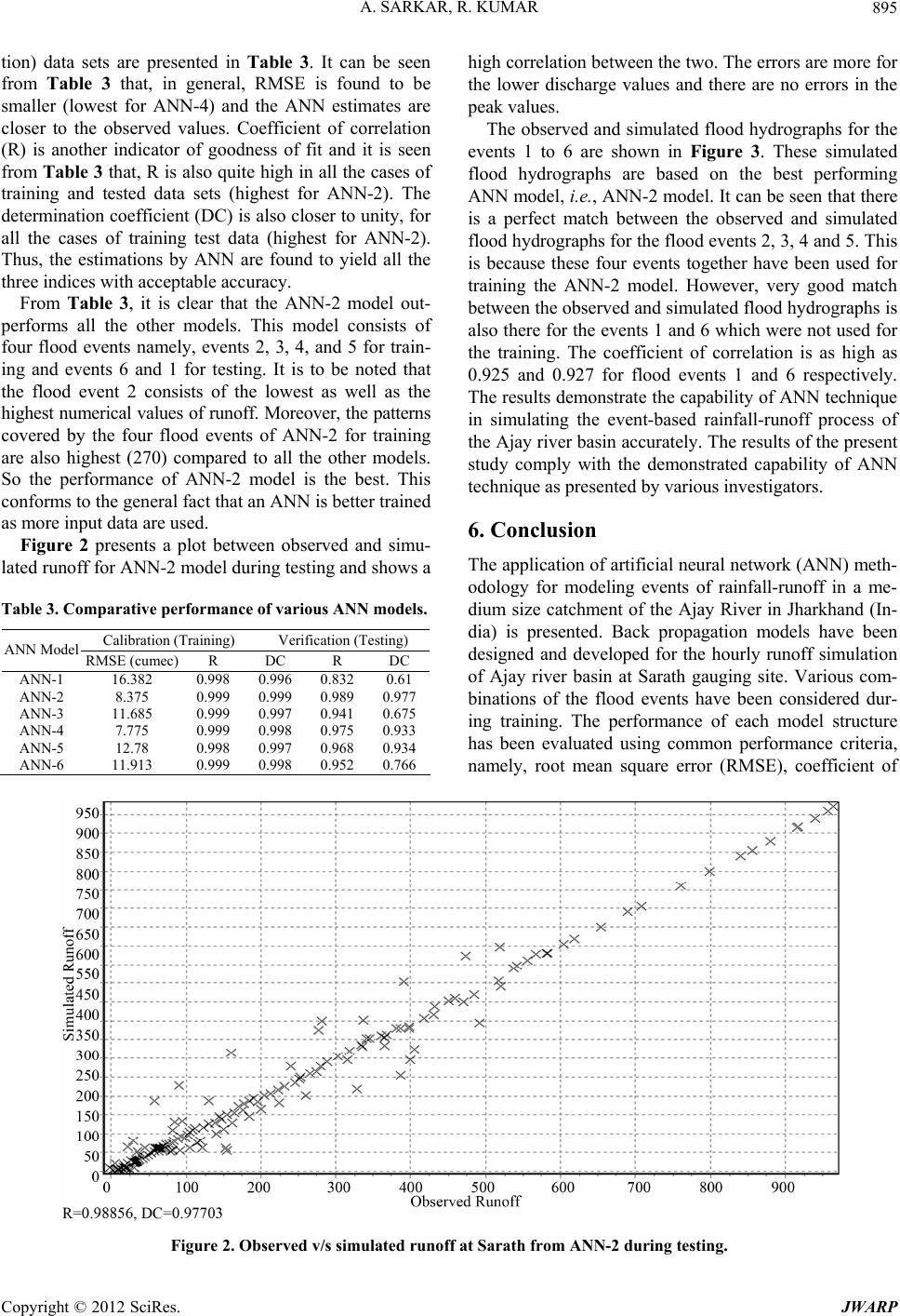

A. SARKAR, R. KUMAR 895

tion) data sets are presented in Table 3. It can be seen

from Table 3 that, in general, RMSE is found to be

smaller (lowest for ANN-4) and the ANN estimates are

closer to the observed values. Coefficient of correlation

(R) is another indicator of goodness of fit and it is seen

from Table 3 that, R is also quite high in all the cases of

training and tested data sets (highest for ANN-2). The

determination coefficient (DC) is also closer to unity, for

all the cases of training test data (highest for ANN-2).

Thus, the estimations by ANN are found to yield all the

three indices with acceptable accuracy.

From Table 3, it is clear that the ANN-2 model out-

performs all the other models. This model consists of

four flood events namely, events 2, 3, 4, and 5 for train-

ing and events 6 and 1 for testing. It is to be noted that

the flood event 2 consists of the lowest as well as the

highest numerical values of runoff. Moreover, the patterns

covered by the four flood events of ANN-2 for training

are also highest (270) compared to all the other models.

So the performance of ANN-2 model is the best. This

conforms to the general fact that an ANN is better trained

as more input data are used.

Figure 2 presents a plot between observed and simu-

lated runoff for ANN-2 model during testing and shows a

Table 3. Comparative performance of various ANN models.

Calibration (Training) Verification (Testing)

ANN Model RMSE (cumec) R DC R DC

ANN-1 16.382 0.9980.996 0.8320.61

ANN-2 8.375 0.9990.999 0.9890.977

ANN-3 11.685 0.9990.997 0.9410.675

ANN-4 7.775 0.9990.998 0.9750.933

ANN-5 12.78 0.9980.997 0.9680.934

ANN-6 11.913 0.9990.998 0.9520.766

high correlation between the two. The errors are more for

the lower discharge values and there are no errors in the

peak values.

The observed and simulated flood hydrographs for the

events 1 to 6 are shown in Figure 3. These simulated

flood hydrographs are based on the best performing

ANN model, i.e., ANN-2 model. It can be seen that there

is a perfect match between the observed and simulated

flood hydrographs for the flood events 2, 3, 4 and 5. This

is because these four events together have been used for

training the ANN-2 model. However, very good match

between the observed and simulated flood hydrographs is

also there for the events 1 and 6 which were not used for

the training. The coefficient of correlation is as high as

0.925 and 0.927 for flood events 1 and 6 respectively.

The results demonstrate the capability of ANN technique

in simulating the event-based rainfall-runoff process of

the Ajay river basin accurately. The results of the present

study comply with the demonstrated capability of ANN

technique as presented by various investigato rs.

6. Conclusion

The application of artificial neural network (ANN) meth-

odology for modeling events of rainfall-runoff in a me-

dium size catchment of the Ajay River in Jharkhand (In-

dia) is presented. Back propagation models have been

designed and developed for the hourly runoff simulation

of Ajay river basin at Sarath gauging site. Various com-

binations of the flood events have been considered dur-

ing training. The performance of each model structure

has been evaluated using common performance criteria,

namely, root mean square error (RMSE), coefficient of

Figure 2. Observed v/s simulated runoff at Sarath from ANN-2 during testing.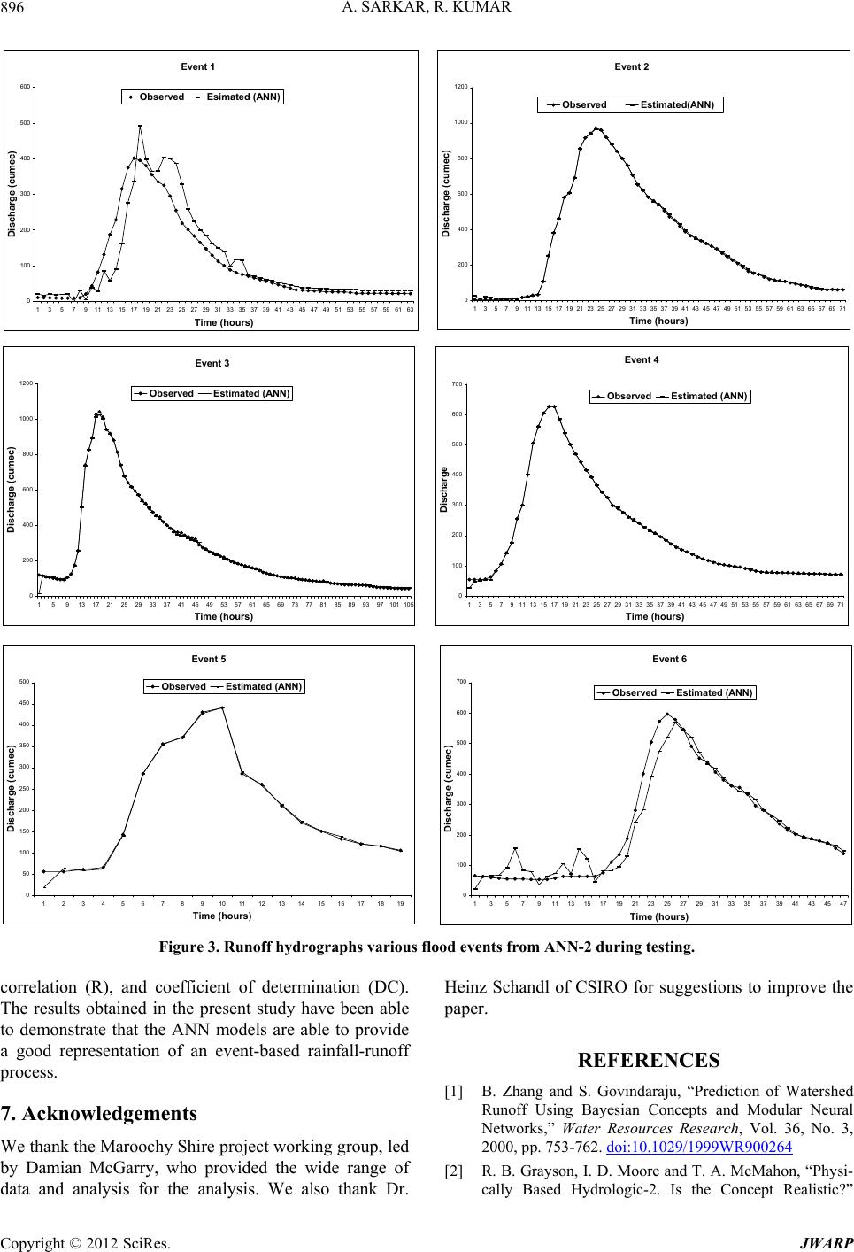

A. SARKAR, R. KUMAR

896

Even t 1

100

200

300

400

500

600

1357911 13 15 17 19 21 23 25 27 29 31 33 35 37 39 41 43 45 47 49 51 53 55 57 59 61 63

Time (hours)

Discharge (cumec)

Observed Esimated (ANN)

Event 2

200

400

600

800

1000

1200

1357911131517192123252729313335373941434547495153

Time (hours)

Discharge (cumec)

555759616365676971

Observed Estimated(ANN)

Event 3

200

400

600

800

1000

1200

159 13172125293337414549535761656973778185899397101105

Time (hours)

Discharge (cumec)

Observed Estimated (ANN)

Event 4

100

200

300

400

500

600

700

1357911131517192123252729313335373941434547495153

Time (hours)

Discharge

555759616365676971

ObservedEstimated (ANN)

Event 5

100

150

200

250

300

350

400

450

500

1 2345678 910111213141516171819

Time (hours)

Discharge (cumec)

ObservedEstimated (ANN)

Event 6

100

200

300

400

500

600

700

1357911131517192123252729313335

Time (hours)

Discharge (cumec)

373941434547

Observed Estimated (ANN)

Figure 3. Runoff hydrographs various flood events from ANN-2 during testing.

correlation (R), and coefficient of determination (DC).

The results obtained in the present study have been able

to demonstrate that the ANN models are able to provide

a good representation of an event-based rainfall-runoff

process.

7. Acknowledgements

We thank the Maroochy Shire project working group, led

by Damian McGarry, who provided the wide range of

data and analysis for the analysis. We also thank Dr.

Heinz Schandl of CSIRO for suggestions to improve the

paper.

REFERENCES

[1] B. Zhang and S. Govindaraju, “Prediction of Watershed

Runoff Using Bayesian Concepts and Modular Neural

Networks,” Water Resources Research, Vol. 36, No. 3,

2000, pp. 753-762. doi:10.1029/1999WR900264

[2] R. B. Grayson, I. D. Moore and T. A. McMahon, “Physi-

cally Based Hydrologic-2. Is the Concept Realistic?”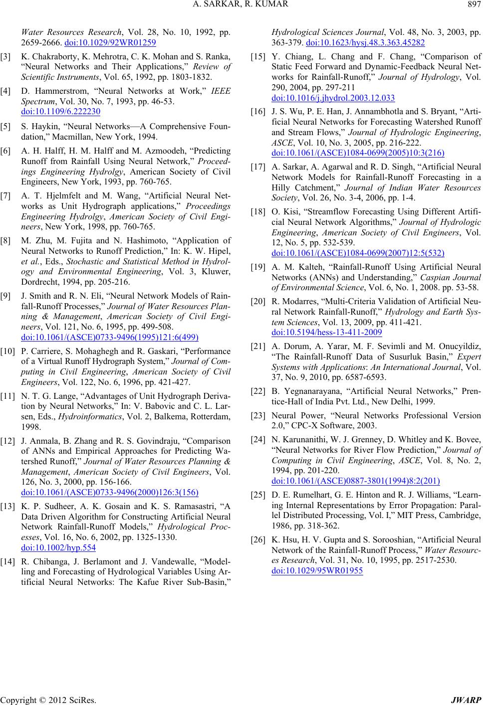

A. SARKAR, R. KUMAR 897

Water Resources Research, Vol. 28, No. 10, 1992, pp.

2659-2666. doi:10.1029/92WR01259

[3] K. Chakraborty, K. Mehrotra, C. K. Mohan and S. Ranka,

“Neural Networks and Their Applications,” Review of

Scientific Instruments, Vol. 65, 1992, pp. 1803-1832.

[4] D. Hammerstrom, “Neural Networks at Work,” IEEE

Spectrum, Vol. 30, No. 7, 1993, pp. 46-53.

doi:10.1109/6.222230

[5] S. Haykin, “Neural Networks—A Comprehensive Foun-

dation,” Macmillan, New York, 1994.

[6] A. H. Halff, H. M. Halff and M. Azmoodeh, “Predicting

Runoff from Rainfall Using Neural Network,” Proceed-

ings Engineering Hydrolgy, American Society of Civil

Engineers, New York, 1993, pp. 760-765.

[7] A. T. Hjelmfelt and M. Wang, “Artificial Neural Net-

works as Unit Hydrograph applications,” Proceedings

Engineering Hydrolgy, American Society of Civil Engi-

neers, New York, 1998, pp. 760-765.

[8] M. Zhu, M. Fujita and N. Hashimoto, “Application of

Neural Networks to Runoff Prediction,” In: K. W. Hipel,

et al., Eds., Stochastic and Statistical Method in Hydrol-

ogy and Environmental Engineering, Vol. 3, Kluwer,

Dordrecht, 1994, pp. 205-216.

[9] J. Smith and R. N. Eli, “Neural Network Models of Rain-

fall-Runoff Processes,” Journal of Water Resources Plan-

ning & Management, American Society of Civil Engi-

neers, Vol. 121, No. 6, 1995, pp. 499-508.

doi:10.1061/(ASCE)0733-9496(1995)121:6(499)

[10] P. Carriere, S. Mohaghegh and R. Gaskari, “Performance

of a Virtual Run off Hydrograph Sy stem,” Journal of Com-

puting in Civil Engineering, American Society of Civil

Engineers, Vol. 122, No. 6, 1996, pp. 421-427.

[11] N. T. G. Lange, “Advantages of Unit Hydrograph Deriva-

tion by Neural Networks,” In: V. Babovic and C. L. Lar-

sen, Eds., Hydroinformatics, Vol. 2, Balkema, Rotterdam,

1998.

[12] J. Anmala, B. Zhang and R. S. Govindraju, “Comparison

of ANNs and Empirical Approaches for Predicting Wa-

tershed Runoff,” Journal of Water Resources Planning &

Management, American Society of Civil Engineers, Vol.

126, No. 3, 2000, pp. 156-166.

doi:10.1061/(ASCE)0733-9496(2000)126:3(156)

[13] K. P. Sudheer, A. K. Gosain and K. S. Ramasastri, “A

Data Driven Algorithm for Constructing Artificial Neural

Network Rainfall-Runoff Models,” Hydrological Proc-

esses, Vol. 16, No. 6, 2002, pp. 1325-1330.

doi:10.1002/hyp.554

[14] R. Chibanga, J. Berlamont and J. Vandewalle, “Model-

ling and Forecasting of Hydrological Variables Using Ar-

tificial Neural Networks: The Kafue River Sub-Basin,”

Hydrological Sciences Journal, Vol. 48, No. 3, 2003, pp.

363-379. doi:10.1623/hysj.48.3.363.45282

[15] Y. Chiang, L. Chang and F. Chang, “Comparison of

Static Feed Forward and Dynamic-Feedback Neural Net-

works for Rainfall-Runoff,” Journal of Hydrology, Vol.

290, 2004, pp. 297-211

doi:10.1016/j.jhydrol.2003.12.033

[16] J. S. Wu, P. E. Han, J. Annambhotla and S. Bryant, “Arti-

ficial Neural Networks for Forecasting Watershed Runoff

and Stream Flows,” Journal of Hydrologic Engineering,

ASCE, Vol. 10, No. 3, 2005, pp. 216-222.

doi:10.1061/(ASCE)1084-0699(2005)10:3(216)

[17] A. Sarkar, A. Agarwal and R. D. Singh, “Artificial Neural

Network Models for Rainfall-Runoff Forecasting in a

Hilly Catchment,” Journal of Indian Water Resources

Society, Vol. 26, No. 3-4, 2006, pp. 1-4.

[18] O. Kisi, “Streamflow Forecasting Using Different Artifi-

cial Neural Network Algorithms,” Journal of Hydrologic

Engineering, American Society of Civil Engineers, Vol.

12, No. 5, pp. 532-539.

doi:10.1061/(ASCE)1084-0699(2007)12:5(532)

[19] A. M. Kalteh, “Rainfall-Runoff Using Artificial Neural

Networks (ANNs) and Understanding,” Caspian Journal

of Environmental Science, Vol. 6, No. 1, 2008. pp. 53-58.

[20] R. Modarres, “Multi-Criteria Validation of Artificial Neu-

ral Network Rainfall-Runoff,” Hydrology and Earth Sys-

tem Sciences, Vol. 13, 2009, pp. 411-421.

doi:10.5194/hess-13-411-2009

[21] A. Dorum, A. Yarar, M. F. Sevimli and M. Onucyildiz,

“The Rainfall-Runoff Data of Susurluk Basin,” Expert

Systems with Applications: An International Journal, Vol.

37, No. 9, 2010, pp. 6587-6593.

[22] B. Yegnanarayana, “Artificial Neural Networks,” Pren-

tice-Hall of India Pvt. Ltd., New Delhi, 1999.

[23] Neural Power, “Neural Networks Professional Version

2.0,” CPC-X Software, 2003.

[24] N. Karunanithi, W. J. Grenney, D. Whitley and K. Bovee,

“Neural Networks for River Flow Prediction,” Journal of

Computing in Civil Engineering, ASCE, Vol. 8, No. 2,

1994, pp. 201-220.

doi:10.1061/(ASCE)0887-3801(1994)8:2(201)

[25] D. E. Rumelhart, G. E. Hinton and R. J. Williams, “Le arn -

ing Internal Representations by Error Propagation: Paral-

lel Distributed Processing, Vol. I ,” MIT Press, Cambridge,

1986, pp. 318-362.

[26] K. Hsu, H. V. Gupta and S. Sorooshian, “Artificial Neural

Network of the Rainfall-Runoff Process,” Water Resourc-

es Research, Vol. 31, No. 10, 1995, pp. 2517-2530.

doi:10.1029/95WR01955