A Rainfall Distribution for the Lampao Site in the Chi River Basin, Thailand

doi:10.4236/jwarp.2012.410101

Paper Menu >>

Journal Menu >>

Journal of Water Resource and Protection, 2012, 4, 866-869

http://dx.doi.org/10.4236/jwarp.2012.410101 Published Online October 2012 (http://www.SciRP.org/journal/jwarp)

A Rainfall Distribution for the Lampao Site in the

Chi River Basin, Thailand

Bungon Kumphon1*, Arun Kaew-Man1, Parakorn Seenoi2

1Department of Mathematics, Mahasarakha m Unive rsity, Mahasarakham, Thailand

2Department of Statistics, Khon Kaen University, Khon Kaen, Thailand

Email: *[email protected]

Received August 12, 2012; revised September 10, 2012; accepted October 11, 2012

ABSTRACT

In this study, the four-parameter kappa distribution with L-Moments estimation has been used to fit the distribution of

weekly rainfall data at Lampao in the Chi River Basin, Thailand. The weekly precip itations with probabilit ies 0.75 were

estimated, and the extreme rainfall estimates obtained can be used for water and agriculture management.

Keywords: L-Moments; Four Parameters Kappa Distribution; Goodness of Fit Test

1. Introduction

This paper deals with precipitation frequency analysis in

the central area of Northeast Thailand. Under the Koppen

classification the Northeast climate is called tropical

wet-dry or tropical savannah. The two main mechanisms

that support the rainfall in this region are the southwest

monsoon during May to October, and the tropical cy-

clone depression July to September. Both are more im-

portant for agriculture and in the design and con struction

of various flood control measures, including the

operational management of reservoirs. Reliable estimates

of rainfall quantities at specified recurrence intervals by

operational hydro-meteo-rologists have therefore been

one issue. Ref [1] investigated the distribution of

monthly rainfall in Northeast Thailand, and found the

data could be fitted by either a Gamma distribution or a

log-normal distribution. A more recent study by [2]

showed that the incomplete Gamma distribution fits the

daily rainfall in Thailand, where the rainfall starts from

week 12 up to between week 20 and week 29, and then

increases up to between week 36 and week 39, with very

heavy rainfall in the Northeast, East and Southern

regions.

In general, maximum likelihood estimation (MLE) is

too sensitive to investigate extreme values. From our

experience with a quasi-Newton algorithm, we find that a

term in the logarithm function goes negative at some

points xi, and the MLE is computationally inefficient.

The L-Moments approach developed by [3] has been

widely used for parameter estimation because it provides

robust and reliable parameter estimation, particularly

from small samples. It is also computationally more trac-

table than MLE, and less sensitiv e to outliers that may be

present in the sample due to severe drought, flood or

cyclone events. Further, L-Moments are linear combin-

ations of ranked observations and do not involve squares

or cubes, as in the more conventional methods for mom-

ent estimators. The four-parameter kappa distribution

(K4D) also introduced by [4] is a very general distribu-

tion form that includes a variety of distributions—e.g. the

generalized extreme value distribution, the generalized

Pareto distribution, the generalized logistic distribution,

the Gumbel distribution, etc. Several applications and

examples see [5-7]. Ref [8] also used the K4D with L-

Moments estimation (L-ME), in modelling Indian mon-

soon rainfall. Ref [9] found that L-ME and MLE work-

ed equally well for the three parameter kappa distribu-

tion.

The K4D with L-Moments procedure is adopted in this

paper, to fit the distribution for the rainfall in a part of the

Chi River Basin—more precisely, on the weekly preci-

pitation data between 1984 to 2010 for the upper North

Eastern region, obtained at the Lampao telemetering

information station and the remote station s of the Hydro-

logy and Water Management Center, Royal Irrigation

department (HWMC) located around the Lampao reser-

voir area. The set of 0.75 probability estimates of the

rainfall then obtained for each week are applicable to

crop water management.

2. Study Area and Data

The Lampao River is a branch of the Chi River, and ex-

tends for 262 km but carries rather little water—viz. ap-

*Corresponding a uthor.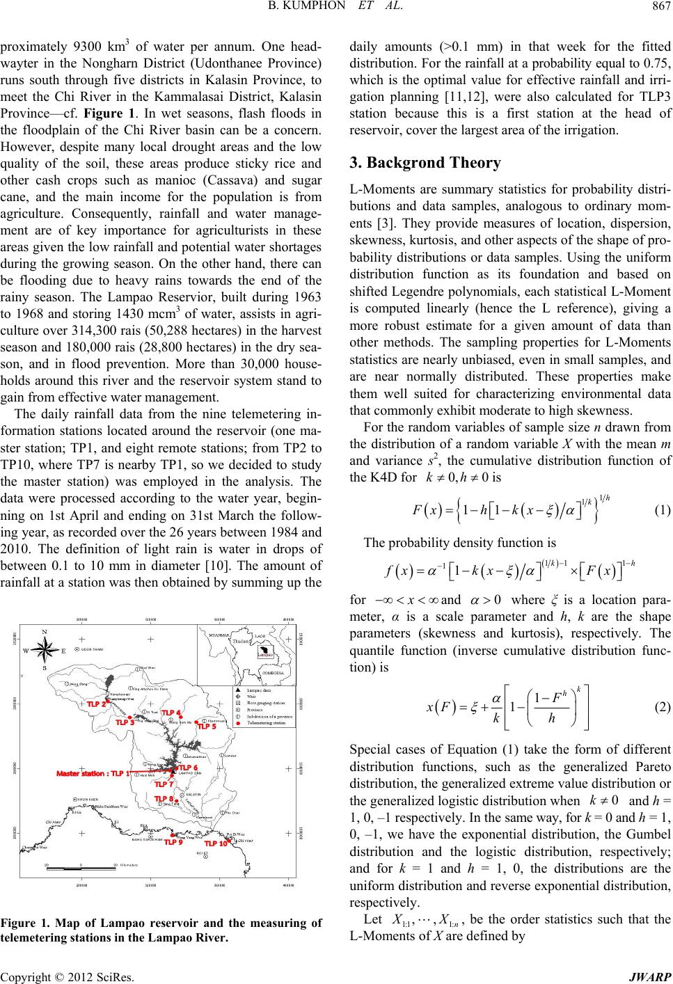

B. KUMPHON ET AL. 867

proximately 9300 km3 of water per annum. One head-

wayter in the Nongharn District (Udonthanee Province)

runs south through five districts in Kalasin Province, to

meet the Chi River in the Kammalasai District, Kalasin

Province—cf. Figure 1. In wet seasons, flash floods in

the floodplain of the Chi River basin can be a concern.

However, despite many local drought areas and the low

quality of the soil, these areas produce sticky rice and

other cash crops such as manioc (Cassava) and sugar

cane, and the main income for the population is from

agriculture. Consequently, rainfall and water manage-

ment are of key importance for agriculturists in these

areas given the low rainfall and potential water shortag es

during the growing season. On the other hand, there can

be flooding due to heavy rains towards the end of the

rainy season. The Lampao Reservior, built during 1963

to 1968 and storing 1430 mcm3 of water, assists in agri-

culture over 314,3 00 rais (50,288 hectares) in the h arvest

season and 180,000 rais (28 ,800 hectares) in the dry sea-

son, and in flood prevention. More than 30,000 house-

holds around this river and the reservoir system stand to

gain from effective water management.

The daily rainfall data from the nine telemetering in-

formation stations located around the reservoir (one ma-

ster station; TP1, and eight remote stations; from TP2 to

TP10, where TP7 is nearby TP1, so we decided to study

the master station) was employed in the analysis. The

data were processed according to the water year, begin-

ning on 1st April and ending on 31st March the follow-

ing year, as recorded over the 26 years between 1984 and

2010. The definition of light rain is water in drops of

between 0.1 to 10 mm in diameter [10]. The amount of

rainfall at a station was then obtained by summing up the

Figure 1. Map of Lampao reservoir and the measuring of

telemetering stations in the Lampao River.

daily amounts (>0.1 mm) in that week for the fitted

dis tribu tion . For the rainfall at a probability equal to 0.75,

which is the optimal value for effective rainfall and irri-

gation planning [11,12], were also calculated for TLP3

station because this is a first station at the head of

reservoir, cover the largest area of the irrigation.

3. Backgrond Theory

L-Moments are summary statistics for probability distri-

butions and data samples, analogous to ordinary mom-

ents [3]. They provide measures of location, dispersion,

skewness, kurtosis, and other aspects of the shape of pr o-

bability distributions or data samples. Using the uniform

distribution function as its foundation and based on

shifted Legendre polynomials, each statistical L-Moment

is computed linearly (hence the L reference), giving a

more robust estimate for a given amount of data than

other methods. The sampling properties for L-Moments

statistics are nearly unbiased, even in small samples, and

are near normally distributed. These properties make

them well suited for characterizing environmental data

that commonly exhibit moderate to high skewness.

For the random variables of sample size n drawn from

the distribution of a random variable X with the mean m

and variance s2, the cumulative distribution function of

the K4D for 0, 0kh



is

 





11 h

Fxh kx



 







(1)

The probability density function is

 



11 1

11kh

fx kxFx







 









for



 and 0



 where ξ is a location para-

meter, α is a scale parameter and h, k are the shape

parameters (skewness and kurtosis), respectively. The

quantile function (inverse cumulative distribution func-

tion) is



xF kh

















 













(2)

Special cases of Equation (1) take the form of different

distribution functions, such as the generalized Pareto

distribution, the generalized ex treme value distribution or

the generalized logistic d istribution wh en and h =

1, 0, –1 respectively. In the same way, for k = 0 and h = 1,

0, –1, we have the exponential distribution, the Gumbel

distribution and the logistic distribution, respectively;

and for k = 1 and h = 1, 0, the distributions are the

uniform distribution and reverse exponential distribution,

respectively.

0k

Let 1:1 1:

,,n

X, be the order statistics such that the

L-Moments of X are defined by

B. KUMPHON ET AL.

868



rrkr

rEXr











 







1,2,

where r is the rth L-Moment of a distribution and E(Xi:r)

is the expected value of the ith smallest observation in a

sample of size r. The first four L-Moments of a random

variable X can be written as



22:21:2

33:32:3 1:3

44:43:42:4 1:4

12,

133 .

EX X

EXX X

EXXX X











[3] demonstrated the utility of estimators based on the

L-Moment ratios in hydrological extreme analysis. The

second moment is often scaled by the mean, so that a

coefficient of variability is determined—viz,









 

where 1



is the measure of location. As with the defi-

nitions and the meaning of the ratios between ordinary

moments, the coefficients of L-kurtosis and L-skew-

ness are defined as







 for , where3r3



is the

measure of skewness (L-Cs) and 4



is the measure of

kurtosis (L-Ck).

4. Application to Weekly Rainfall

The exact distribution of parameter estimators obtained

by this method is difficult to derive in general, so we ex-

plored the fit between the theoretical distribution (K4D)

and the real data set, as shown in Figure 2. Parameters

and a goodness of fit test via the Kolmogorov-Smirnov-

test (KS) and the Anderson-Darling test (AD) with a 0.05

significance level computed for the data at all nine

stations are tabulated in Table 1 and shown that K4D fit

well with all the rainfall for nine stations. A close inspec-

tion of the parameters shows values of the respective

parameters h > 0 and , suggesting that the underly-

ing distribution tends towards the generalized Pareto

distribution rather than the generalized extreme value

distribution fo r all stations.

0k

As an application of this methodology to the estima-

tion of the maximum amount of rainfall at the 0.75 prob-

ability each week, the example observations were shown

at one station above the reservoir within the Chi Basin

using the parameters in Equations (1) and (2) estimated

at TLP3 station. The estimated values have been

computed as presented in Table 2. The highlighted area

Figure 2. The exploration for goodness of fit for K4D at

TLP3 station.

Table 1. Parameters estimation and goodness of fit test for

the K4D distribution.

site locationscaleh k KS (p-value) AD (p-value)

TLP1–23.355169.4270.2731.165 0.280 (0.953 ) 0.0402 (0.887)

TLP2–14.444176.8330.3211.088 0.240 (0.975 ) 0.0360 (0.943)

TLP3–37.121237.3760.4551.127 0.061 (0.26 7) 1.370 (0.211)

TLP4–18.790178.1920.2921.101 0.320 (0.923 ) 0.031 (0.988)

TLP5–18.872166.9700.3781.121 0.243 (0.974 ) 0.031 (0.990)

TLP626.010146.2380.2830.787 0.535 (0.711) 0.037 (0.933)

TLP826.051112.9080.1570.731 0.3880 (0.861) 0.040 (0.943)

TLP920.012152.2460.2940.819 0.717 (0.544) 0.043 (0.812)

TLP 1048.534117.7650.1360.538 1.101 (0.308) 0.051 (0.649)

Table 2. The estimation of the maximum amount of rainfall

for each week at the 0.75 probability, TLP3 station.

Week AmountWeek Amount Week Amount

1 0.000 19 61.487 37 73.535

2 0.000 20 61.835 38 62.461

3 0.000 21 76.256 39 37.234

4 0.000 22 69.715 40 49.580

5 0.305 23 65.838 41 39.601

6 0.000 24 72.143 42 22.817

7 1.566 25 74.050 43 4.943

8 0.000 26 60.660 44 4.855

9 5.483 27 64.666 45 0.000

10 0.000 28 56.508 46 0.039

11 1.659 29 65.155 47 0.000

12 16.165 30 41.593 48 0.000

13 23.785 31 79.242 49 0.000

14 10.443 32 82.184 50 0.000

15 16.638 33 103.833 51 0.000

16 19.828 34 103.358 52 0.000

17 43.136 35 84.370

18 45.875 36 110.496

shows the rainy season from week 19 to week 40. The

K4D realdata

B. KUMPHON ET AL.

869

awareness weeks are weeks 33 to 36, with very heavy

rain (84 to 110 mm.). This is useful information for the

hydro-meteorologists, and for reservoir planners who

manage water release and storage before and during the

awareness weeks 33 to 36. The best weeks for agri-

culturists to plan drying processes for crops are 1 to 6, 8,

10 and 45 to 52 because there is then no rainfall.

5. Conclusion

For the planning and design of crop scheduling and the

design of water management in Northeast Thailand, the

distribution of weekly rainfall was investigated from data

on weekly rainfall for a part of Chi River Basin sur-

rounding the Lampao Reservoir. The data is fitted well

by K4D with L-Moments estimation, and there is some

evidence for a generalized Pareto distribution. There is

usually one distribution that passes the goodness-of-fit

test. Although, ther e might be more than one distribu tion

for this relatively small region (from the family of such

distributions). For the estimated rainfall at the specific

probability 0.75, there is low to no rainfall in the dry

season, which is the best time for drying crops or any

associated activity that has no water requirement. On the

other hand, there is very high value of rainfall in the

rainy season.

6. Acknowledgements

Financ ial support was provided by the Faculty of Scienc e ,

and Mahasarakham University Development Fund, Maha-

sarakham University. The data was provided by the Hy-

drology and Water Management Center for the upper

north eastern Royal Irrigation department, Thailand. The

author thanks Professor Roger Hosking for his support

and helpful suggestions.

REFERENCES

[1] H. N. Phien, A. Arbhabhirama and A. Sunchindah, “Dis-

tribution of Monthly Rainfall in Northeast Thailand,”

Southeast Asian Studies, Vol. 18, No. 1, 1980, pp. 110-

122.

[2] A. Phayomjamsri, “Weekly Rainfall Probability for Thai-

land,” Study and Research Division, Meteorological Da-

partment, Bangkok, 2008.

[3] J. R. M. Hosking, “L-Moments: Analysis and Estimation

of Distribution Using Linear Combination of Order Sta-

tistics,” Journal of the Royal Statistical Society Series B,

Vol. 52, No. 1, 1990, pp. 105-124.

[4] J. R. M. Hosking, “The Four-Parameter Kappa Distribu-

tion,” IBM Journal of Research Development, Vol. 38,

No. 3, 1994, pp. 251-258. doi:10.1147/rd.383.0251

[5] E. S. S. Eslamian and H. Feizih, “Maximum Monthly

Rainfall Analysis Using L-Moments for an Arid Region

in Isfahan Province, Iran,” Journal of Applied Meteorol-

ogy and Climatology, Vol. 46, 2007, pp. 494-503.

doi:10.1175/JAM2465.1

[6] J. S. Park and H. S. Jung, “Modelling Korean Extreme

Rainfall Using a Kappa Distribution,” Biometrika, Vol.

79, 2002, pp. 827-832.

[7] J. R. M. Hosking and J. R. Wallis, “Regional Frequency

Analysis. An Approach Based on L-Moments,” Cam-

bridge University Press, Cambridge, New York, Mel-

bourne, 1997. doi:10.1017/CBO9780511529443

[8] B. P. Parida, “Modelling of Indian Summer Monsoon

Rainfall Using a Four-Parameter Kappa Distribution,”

International Journal of Climatology, Vol. 19, No. 12,

1999, pp. 1389-1398.

doi:10.1002/(SICI)1097-0088(199910)19:12<1389::AID-

JOC435>3.0.CO;2-T

[9] J. S. Park, S. C. Seo and T. Y. Kim, “A Kappa Distribu-

tion with a Hydrological Application,” Stochastic Envi-

ronmental Research and Risk Assessment, Vol. 23, No. 5,

2009, pp. 579-586. doi:10.1007/s00477-008-0243-5

[10] Thai Meteorological Department, “Thai Weather,” 2007.

http://www.tmd.go.th/info/info.php?FileID=22

[11] N. G. Dastane, “Effective Rainfall in Irrigated Agricul-

ture,” FAO Irrigation, and Dr ainage Pape r No. 25, Rome,

1977.

[12] L. R. Oldeman and M. Frere, “A Study of the Agrocli-

matology of the Humid Tropics of Southeast Asia,” Tech-

nical Note No. 179, Food and Agriculture Organisation of

the United Nations, 1982, pp. 72-76.