On a New Method of N-Body Simulations

doi:10.4236/ijaa.2012.23015

Paper Menu >>

Journal Menu >>

International Journal of Astronomy and Astrophysics, 2012, 2, 113-118

http://dx.doi.org/10.4236/ijaa.2012.23015 Published Online September 2012 (http://www.SciRP.org/journal/ijaa)

On a New Method of N-Body Simulations

E. Vilkoviskij

Fesenkov Astrophysical Institute, Observatory, Almaty, Kazakhstan

Email: [email protected]

Received July 4, 2012; revised August 15, 2012; accepted August 30, 2012

ABSTRACT

The theoretical foundation of a new N-body simulation method for the dynamics of large numbers (N > 106) of gravi-

tating bodies is described. The new approach is founded on the probability description of the physical parameters and a

similarity method which permits a manifold reduction of the calculation time for the evolution of “large” systems. This

is done by averaging the results of calculations over an ensemble of many “small” systems with total particle number in

the ensemble equal to the number of stars in the large system. The method is valid for the approximate calculation of

the evolution of large systems, including dissipative systems like AGN containing a super-massive black hole, accretion

disc, and the surrounding stellar cluster.

Keywords: Galaxies; Nuclei; Methods; N-Body Simulations

1. Introduction

At present the methods of modeling systems of many

gravitating bodies have been highly refined, but appli-

cation of these methods to the calculation of very large

systems containing N ~ 106 - 1011 stars (large globular

clusters, galaxies and their active nuclei) faces major

limitations due to limited computer resources. Further-

more, direct calculation of interactions of every pair of

stars demands time proportional to the square of the

number of stars (gravitating bodies) N in the system, the

whole calculation time (with the calculation time ∆t for

every pair) is proportional to Т ~ ∆t(N)2. Usually, one

needs to carry the calculations out to a time of the order

of the relaxation time trx of the system, which is propor-

tional to the number of the gravitating bodies N. Thus the

real “cost” of the calculations behaves as [1]



,rx

TNt tN (1)

Such calculations are difficult or impossible for the

systems with N > 106 due to limited resources of even the

most advanced modern supercomputers, with the fast

processors with about 1 Petaflops (1015 sec−1) [1]. Of

course, now many approximate methods are developed,

such as tree-codes [2], which use the averaged descrip-

tions of the gravity for the distant particle groups. But the

classical task of the “direct” calculations of every pair of

the gravitating bodies keeps its central role as the most

precise method.

In the present paper we discuss a new approximate

method for the acceleration of N-body simulations of

large stellar systems. We refer to it as the Aldar-Kose

method, using the name of a cheery hero of the Kazakh

folklore. We discuss its likely areas of application and

limitations of the method. In the accompanying paper [3]

we show with a sample of simulations, that the method

promises essential acceleration of calculations of the

evolution models of stellar systems and active galactic

nuclei (AGN).

2. Statistical and Dynamical Equivalence of

the Gravitating Systems’ Models with

Different Initial Particles’ Distributions

Any numerical calculation of N-body dynamics has to be

started with definition of the initial coordinates and ve-

locities of all bodies, Xni(t0), Vni(t0), where i = 1, 2, 3

corresponds to the Cartesian coordinates and velocity

projections of every n-th of the total N number of the

bodies at the starting time t0 = 0. This initial distribution

is defined usually with the special procedure of random

numbers’ generation, which represents some initial quasi-

equilibrium (with the given full energy of the system)

distribution function of the bodies in the common gravity

field.

As soon as the initial distributions of the coordinates

and velocities of bodies are determined with a random

numbers’ generation, the condition of the “statistical and

dynamical equivalence” of the solutions is implicitly

used in any numerical simulations. Let us analyze the

concept more distinctly. To avoid non-essential details

we simplify the model task supposing equality of the

masses of the stars and ignoring direct (contact) stellar

collisions, so reducing the task to the “gravitating points”

E. VILKOVISKIJ

114

dynamics. Also, for simplicity, further we will ignore the

problem of “primordial binaries”, supposing that their

number is determined with the random numbers in the

initial conditions.

As the stellar systems are open, the achievement of the

exact equilibrium distribution function of the stars’ ve-

locities (in Boltzmann’s sense) is impossible, because the

tendency to statistical equilibrium leads to dissipation of

stars with large energies, which determines slow evolu-

tion of the system due to the “evaporation” of the stars

and the final collapse of the core of the system. The rate

of the evolution is determined with the relaxation time of

the system [4]



0.14

ln 0.4

rx cr

t



(2)

where N is the total number of stars in the system,

ln(0.4N) is the so-called “Coulomb logarithm” for stellar

systems, tcr—the crossing time, determined usually as the

time needed for a star to cross the region of the system

containing half of the system’s mass. Note that the nume-

rical coefficients in (2) are known with the precision ~

30% - 50% only; here we give the most commonly used

values.

Let us turn back to the question of equivalence of the

evolution processes in the systems with different (in the

sense of different realization of random numbers choos-

ing) initial conditions. Of course, the concrete orbits of

particles in the systems with different initial conditions

will be completely different, but the dynamical behavior

and the secular evolution of the distribution functions of

the physical parameters of the orbits in both systems will

be equivalent in statistical and dynamical sense, if we are

interested of distribution functions, but not of the con-

crete orbits. Note that the quality of modern computers is

such that the orbits of the particles, calculated in two

simulations with the same initial conditions will be ab-

solutely identical. In contrast, in real stellar systems there

are always some random factors, which lead to a mixing

(random small deviations) of the orbits. As a result, the

distribution functions only, not the concrete stellar orbits

may be compared between a model and real systems.

Consequently, one may speak not about identity, but only

about dynamical and statistical equivalence of a model

and real stellar systems. The situation is similar, in a

sense, (not literally!) to the quantum-mechanics des-

cription: Only the probability description is valid, so the

description with a single numerical calculation is “too

much deterministic” and, in that sense, non-adequate

(fuller analyses of some analogies in quantum mechanics

were discussed earlier in [5]).

In fact, the characteristic times of achievement of the

“chaotic” (statistical) equilibrium in stellar systems are

much shorter than the relaxation time (2), due to the

quick dynamical mixture of the systems [6]. As a result,

the solutions with different initial conditions in the same

system (the “microscopically” different solutions) are

supposed to be dynamically and statistically equivalent.

As a rule, the problem of different initial condition (in

the sense of different random realization) is usually even

not discussed, and the solution for the system evolution

is realized with a single initial condition of stars’ (par-

ticles’) coordinates and velocities distribution.

With particle numbers more than several thousands,

the probability of a deviation from “almost equilibrium”

initial distribution is diminishingly small, but the pro-

blem becomes actual for the systems with comparatively

small number of particles, and for the systems feebly

stable relative to the small perturbations. Because of that,

the question of equivalence of the numerical solutions

became important for comparison of the systems with

different numbers of particles, N1 and N2 << N1.

3. The Dynamical Equivalence of the

Systems with Different Particle Numbers

Let us consider the question of the dynamical equiva-

lence of the evolution of two systems with different par-

ticle numbers, N1 and N2 << N1. To compare the relaxa-

tion processes in the systems it is convenient to use di-

mensionless unit system (the N-body units, NBU [4]),

usually employed in model tasks. In these units, the total

mass of the system is M = 1, its characteristic size R = 1,

and the gravitation constant G = 1. In this system, the

characteristic particle velocity is V = (GM/R)1/2 = 1, the

characteristic particle crossing time Tcr = R/V = 1, and

the characteristic time of evolution of the system (the

relaxation time) is



0.14

ln 0.4

 (3)

We define the concept of the dynamical equivalence of

the solutions for the systems with different particle num-

bers. It is naturally to suppose that the behavior of two

systems with different (but large enough) particle num-

bers N1 and N2 N1 will be dynamically equivalent, if

the physical parameters of the systems are compared at

equivalent moments of evolution, defined by equal evo-

lution time of systems Tev = t/Trx. The evolution times are

measured in N-body relaxation time units of both sys-

tems (one may call these units the NBEU, the “N-body

evolution units” system),



2211rxrx ev

tTtT T (4)

In the NBU system, the time (and the relaxation times)

for both systems are defined through the crossing times,

which are equal to unity (Tcr1 = Tcr2 = 1), and in the

NBEU the evolution time is defined through the relaxa-

tion time. The relation of the “equivalent dynamical evo-

E. VILKOVISKIJ 115

lution times” in the NBU system is equal to the relation

of their relaxation times:



111 2

ln 0.4

tT NN

 (5)

In the NBU system, the sizes and dynamical parameters

of stellar systems are equal, but the particles in the small

(N2) system have masses m2 = m1N1/N2, and the volume

densities of the particles relate as N1/N2. As a result, the

crossing times are equal, and the NBU dynamical evo-

lution times in the systems are related as (5). In the NBEU,

the time units are relaxation times, so the evolution time of

systems in equal (identical) moments of evolution is

universal, Tev = Tev1 = Tev2.

The stellar dynamics in star systems is defined with

superposition of two processes: The motion along the

“smooth” orbits in the averaged gravitation field of the

system, and the “quasi-Brownian” motion as the result of

random approaches of stars and their density fluctuations.

From (4) and (5) it follows that independently of the par-

ticle numbers in the systems, their dynamical properties

and the time behavior of the physical parameters will be

dynamically equivalent in identical moments of the evo-

lutions Tev, defined through the relaxation times of both

similar systems.

4. The Scaling Coefficient of the Dynamical

Equation for the Dissipative Systems with

Different Particle Numbers

Let us consider the behavior of the stellar systems in the

presence of dissipative processes. For definiteness, let it

be the active galactic nuclei (AGN), consisting of the

compact stellar cluster (CSC) with mass M, the central

super-massive black hole (BH) with mass МBH = 0.1М,

and the accretion disc (AD) with the mass Мd = 0.01М,

surrounding the BH. The model is, as they say, the “toy”

one—in the sense that the disc parameters (the mass and

the rotating moment) are considered to be constants, in

spite of the star-disk interactions and the gas and star

accretion to the BH; so the total mass and the total rotat-

ing moment of the system are not conserved—but it is

not important for the further comparative analyses of the

N-body tasks (one can imagine that the accretion disk is

fed by gas from the outer “obscuring torus” of the AGN).

The dynamics of the system, besides the star-star pair

interaction, will be defined with gravitation of the black

hole and the dissipative star-disk interactions [7]. In the

simplest case, the last one is reduced to a friction force,

which is directed opposite to the velocity of the star re-

lative to the gas in the disk Vsd and is proportional to the

square of the velocity, the square of the stellar radius Rs

and the gas density ρ(r). So, the dissipative force is



ssdsd

QR r



FV

where Vsd = Vs – Vd is the (vector) difference of the star

and gas velocities, Vsd is the module of the velocity, and

Q is a coefficient of the order of 10.

In a typical AGN, the mass of the CSC is М ~ 108 MS,

(of the solar masses), and the number of stars in the sys-

tem are N1 ~ 108. Let us compare the evolution of this

“large” (real) system (N1 stars with masses MS = M/N1) to

the evolution of a similar “small” (the representing) sy-

stem with the number of particles N2 = N1/m and with the

same subsystem’s mass relations as in the large one. In

NBU, the masses of the particles M2 = mM1, and the

sizes and masses of subsystems are the same as in the

large AGN system, with the total masses normalized to 1.

The dissipative acceleration per unit mass in the NBU

has to be the same in both systems to keep the net velo-

city change of a particle per disk crossing independent of

m = N1/N2 (one can imagine that groups of m = N1/N2

stars are decelerated coherently in the small system). So,

the dissipative accelerations of the particles are the same

in the both systems,



sd sds

aQR rM



 V (6)

Now, to compare evolution of the small and large sys-

tems, we have to take into account also the difference

between the relaxation times in both systems, to keep the

dissipative and relaxation time-scales comparable. As in

the NBU all sizes and masses of the subsystems (i.e.

CSC, BH and AD), as well as the typical velocities of

particles and crossing times are the same in both large

and small systems, it is natural to suppose, that behavior

(the dynamical evolution) of both systems will be dy-

namically equivalent, if we compare them at equal mo-

ments of evolution (4) of both systems. So, we have to

take into account, that the relaxation time in the small

system is diminished as compared to the large system

according to (5). Due to this, to keep the balance between

the effects of the particle-particle and the particle-disk

interactions, we must multiply the dissipative accele-

ration (6) in the small system by the “scaling coefficient”

of similarity, SС = SС(N2,N1), which is equal to the rela-

tion of numbers of the disk crossing events by stars per

their relaxation times in both systems. So, the scaling

coefficient to equalize the dissipative and the relaxation

time scales in the small system is

 



22 1

ln 0.4

,ln 0.4

SC NNTN N

 (7)

The introduction of the SC to the dissipative force to

keep the similarity of evolution of both systems is rea-

sonable at least for the cases when the energy changes of

the particles per crossing time (due to the relaxation pro-

cesses and due to dissipative force per crossing time) are

relatively small both in the “large” and the “small” sy-

stems. This circumstance can limit the relation m = N1/N2

E. VILKOVISKIJ

116

of the particle numbers in the real and the “representing”

model systems.

Now let us take into account that the particle numbers

N2 and N1 in both systems can change in time both be-

cause of the accretion of the stars to the central BH (the

intensity of the process is essentially increased in AGN

as the result of star-disk interactions [7]) and due to the

“evaporation” of the stars from the systems. These ef-

fects can be taken into account with introduction of the

variable relaxation and evolution times. Denoting i = 1, 2

for the large and the small systems, and using t for the

dynamical time, we can write:

 



0.14

ln 0.4

rx i

Tt Nt

 (8)

 



ln 0.4d

0.14

Tt t





 (9)

where













,out,iibhi i

NtN NtNt



 

;





,bh i



and





out,i are the numbers of stars captured to the BH

and evaporated from the systems. Remind that Tev(t) are

equal in both systems by definition.



The time-dependent N1(t) and N2(t) have to be intro-

duced to the SC as well:

 



ln 0.4

SC NtNtTt

Nt Nt



(10)

Here the number N1(t) is present, which is supposed to be

unknown in the A-K model simulation and has to be de-

fined through N2(t). For that, let us transform (10) from

the NBU time units to the evolution time units NBEU,

defined with (9). Then we have















ln 0.4

rx ev

ev ev

SC NNTTT

NT NT



(11)

As, by definition,

 

112 2

ev evevev

NTNTN TN T 0, finally we

have

 



212 2

ln 0.4

,, ln 0.4

SC NNTNNN NT

 (12)

where N1/N2 is the relation of initial particle numbers in

the systems. So, in the approximation, the SC depends on

t very slowly (logarithmically).

Using (12), one can calculate the evolution of the

small system (which “represents” the evolution of the

large system), using only the initial relation of the parti-

cle numbers in both systems, and the universal Tev, equal

in both systems.

Here we can see the meaning of approximating re-

presentation of the large system by the small one: The

small system “represents” the large one, but not literally.

The main difference is that we change many disk-cross-

ing events of small particle in the large system, to one

crossing event (with the SC) of a large particle in the

small system. In the first case the crossing point can

move along the disk radius (due to scattering of the orbits

and small distortion of the spherical symmetry of the BH

potential by the disk gravity), slowly changing the con-

ditions of the crossings. In the “small” system the pro-

cess is changed with one event at the single crossing

point. This difference is the main reason limiting the re-

lation m = N1/N2 (see discussion below in the Part 6 of

the paper).

So, the dynamical equivalence of the small and the

large dissipative systems is approximate only and has to

be carefully controlled. The corresponding scaling coeffi-

cients can be obtained for other processes as well, like

the direct (contact) stellar collisions, stellar evolution and

other processes.

5. The Statistical Equivalence of the

Solutions for the Systems with Different

Numbers of Particles: The Aldar-Kose

Method

It is obvious that the above-described dynamical equi-

valence of the small and the large systems does not mean

the statistical equivalence of the model solutions for them,

because the statistical precisions of the solutions are re-

lated as (N2/N1)1/2. The natural way to increase the statis-

tical precision of solutions for the small systems is the

manifold repeated calculations among the ensemble of

small systems. Providing the simulations of small systems

m = (N1/N2) times with different (randomly defined) ini-

tial conditions, and averaging the results over the full

ensemble of the solutions at identical Tev moments, one

will obtain the demanded increasing of the precision to the

statistical precision, achieved with a single model solution

of one large system.

So, we conclude that the mean values of physical pa-

rameters, obtained with averaging over m = N1/N2 model

solutions for the ensemble of dynamically equivalent

“small” systems (every with N2 particles), are equivalent

to those obtained with one solution for the “large” system

(N1 particles), both in the dynamical and statistical senses.

This conclusion has principal meaning for substanti-

ation of the proposed new method (the A-K method) for

the model simulations of evolution of the stellar systems

and AGN, containing compact stellar clusters. Remind

that the “classical” direct method of the N-body simula-

tions of the systems evolution demands spending of the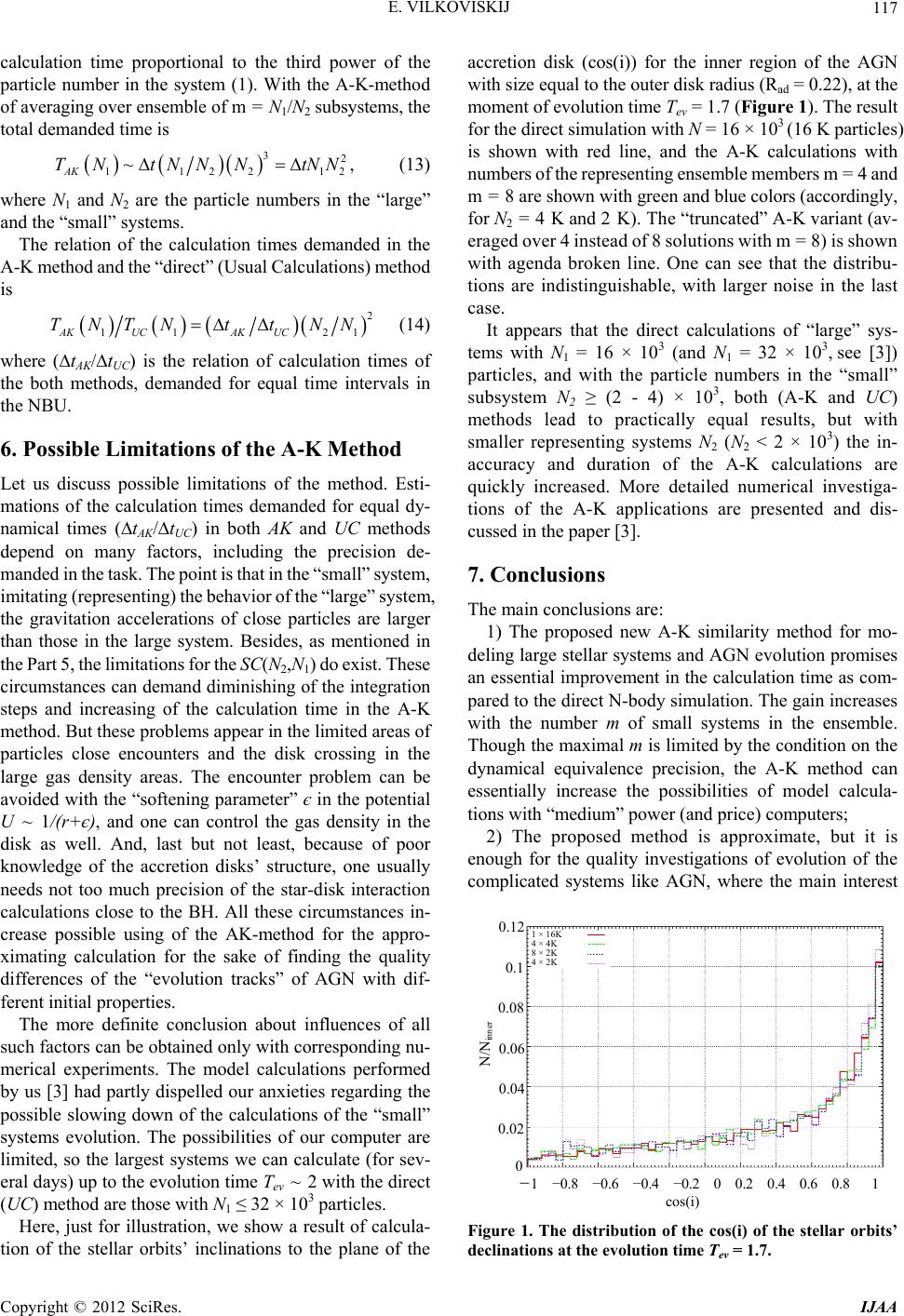

E. VILKOVISKIJ 117

calculation time proportional to the third power of the

particle number in the system (1). With the A-K-method

of averaging over ensemble of m = N1/N2 subsystems, the

total demanded time is

 

1122

TN tNNNtNN

, (13)

where N1 and N2 are the particle numbers in the “large”

and the “small” systems.

The relation of the calculation times demanded in the

A-K method and the “direct” (Usual Calculations) method

 





11 2AKUCAK UC

TNTNtt NN 



(14)

where (∆tАK/∆tUC) is the relation of calculation times of

the both methods, demanded for equal time intervals in

the NBU.

6. Possible Limi t ations of the A-K Method

Let us discuss possible limitations of the method. Esti-

mations of the calculation times demanded for equal dy-

namical times (∆tАK/∆tUC) in both AK and UC methods

depend on many factors, including the precision de-

manded in the task. The point is that in the “small” system,

imitating (representing) the behavior of the “large” system,

the gravitation accelerations of close particles are larger

than those in the large system. Besides, as mentioned in

the Part 5, the limitations for the SC(N2,N1) do exist. These

circumstances can demand diminishing of the integration

steps and increasing of the calculation time in the A-K

method. But these problems appear in the limited areas of

particles close encounters and the disk crossing in the

large gas density areas. The encounter problem can be

avoided with the “softening parameter” є in the potential

U ~ 1/(r+є), and one can control the gas density in the

disk as well. And, last but not least, because of poor

knowledge of the accretion disks’ structure, one usually

needs not too much precision of the star-disk interaction

calculations close to the BH. All these circumstances in-

crease possible using of the AK-method for the appro-

ximating calculation for the sake of finding the quality

differences of the “evolution tracks” of AGN with dif-

ferent initial properties.

The more definite conclusion about influences of all

such factors can be obtained only with corresponding nu-

merical experiments. The model calculations performed

by us [3] had partly dispelled our anxieties regarding the

possible slowing down of the calculations of the “small”

systems evolution. The possibilities of our computer are

limited, so the largest systems we can calculate (for sev-

eral days) up to the evolution time Tev ~ 2 with the direct

(UC) method are those with N1 ≤ 32 × 103 particles.

Here, just for illustration, we show a result of calcula-

tion of the stellar orbits’ inclinations to the plane of the

accretion disk (cos(i)) for the inner region of the AGN

with size equal to the outer disk radius (Rad = 0.22), at the

moment of evolution time Tev = 1.7 (Figure 1). The result

for the direct simulation with N = 16 × 103 (16 K particles)

is shown with red line, and the A-K calculations with

numbers of the representing ensemble members m = 4 and

m = 8 are shown with green and blue colors (accordingly,

for N2 = 4 K and 2 K). The “truncated” A-K variant (av-

eraged over 4 instead of 8 solutions with m = 8) is shown

with agenda broken line. One can see that the distribu-

tions are indistinguishable, with larger noise in the last

case.

It appears that the direct calculations of “large” sys-

tems with N1 = 16 × 103 (and N1 = 32 × 103, see [3])

particles, and with the particle numbers in the “small”

subsystem N2 ≥ (2 - 4) × 103, both (A-K and UC)

methods lead to practically equal results, but with

smaller representing systems N2 (N2 < 2 × 103) the in-

accuracy and duration of the A-K calculations are

quickly increased. More detailed numerical investiga-

tions of the A-K applications are presented and dis-

cussed in the paper [3].

7. Conclusions

The main conclusions are:

1) The proposed new A-K similarity method for mo-

deling large stellar systems and AGN evolution promises

an essential improvement in the calculation time as com-

pared to the direct N-body simulation. The gain increases

with the number m of small systems in the ensemble.

Though the maximal m is limited by the condition on the

dynamical equivalence precision, the A-K method can

essentially increase the possibilities of model calcula-

tions with “medium” power (and price) computers;

2) The proposed method is approximate, but it is

enough for the quality investigations of evolution of the

complicated systems like AGN, where the main interest

1 × 16

4 × 4K

8 × 2K

4 × 2

0.12

0.1

0.08

0.06

0.04

0.02

N/N

inner

−1 −0.8 −0.6 −0.4 −0.2 0 0.2 0.4 0.6 0.8 1

cos(i)

Figure 1. The distribution of the cos(i) of the stellar orbits’

declinations at the evolution time Tev = 1.7.

E. VILKOVISKIJ

118

is the qualitative differences between evolution tracks of

the systems with different initial parameters;

3) Since the statistical precision of solutions for dif-

ferent physical parameters behaves as σ ~ 1/(N1)1/2, the

achievable formal precision of the A-K method is usually

far greater than those obtained from observations. This

permits further optimization of the method using “trun-

cated” A-K method: The number of the small systems for

averaging the physical parameters in the ensemble can be

chosen to be much smaller than m = N1/N2, which further

reduces the demands on calculation time compared to the

“complete” (full) A-K method.

4) Numerical experiments with more powerful compu-

ters are necessary to investigate the exact possibilities

and limits of applications of the method for the solutions

of specific problems of stellar dynamics and AGN evo-

lution.

In conclusion, it should be noted that our formulae (8 -

12) are approximate, as we use the concept of the “total”

relaxation time, which possibly is only approximate when

a stellar system changes its spatial structure and symmetry.

This issue will be investigated in future works.

8. Acknowledgements

The author is grateful to M. A. Makukov for the numeri-

cal calculations (to be published in the accompanying

paper [3]), to I. S. Vilkoviskij for useful discussion of the

variable Tev(t), and to all participants of the “STAR-

DISK” project (P. Berczik, R. Spurzem, Ch. Omarov, M.

Makukov, D. Yurin, A. Just) for the elaboration of the

computer code for the direct N-body simulations of AGN

evolution with a single representing stellar system (m = 1).

REFERENCES

[1] P. Hut, “Dense Stellar Systems as Laboratories for Fun-

damental Physics,” New Astronomy Reviews, Vol. 54, No.

3-6, 2010, pp. 163-172. doi:10.1016/j.newar.2010.09.009

[2] S. Aarseth, “From NBODY1 to NBODY6: The Growth

of an Industry,” The Publications of the Astronomical So-

ciety of the Pacific, Vol. 111, No. 765, 1999, pp. 1333-

1346. doi:10.1086/316455

[3] E. Vilkoviskij and M. Makukov, International Journal of

Astronomy and Astrophysics, 2012.

[4] D. Heggie and P. Hut, “The Gravitational Million-Body

Problem,” Cambridge University Press, Cambridge, 2003.

doi:10.1017/CBO9781139164535

[5] W. Saslaw, “Gravitational Physics of Stellar and Galactic

Systems,” Cambridge University Press, Cambridge, 1987.

[6] D. Lynden-Bell, “Statistical Mechanics of Violent Re-

laxations in Stellar Systems,” Monthly Notices of the

Royal Astronomical Society, Vol. 136, 1967, pp. 101-121.

[7] E. Vilkoviskij and B. Czerny, “The Role of the Central

Stellar Cluster in AGN,” Astronomy and Astrophysics,

Vol. 387, 2002, pp. 804-819.

doi:10.1051/0004-6361:20020255