Flow behavior of UCM viscoelastic fluid in sudden contraction channel

doi:10.4236/ns.2010.27098

Paper Menu >>

Journal Menu >>

Vol.2, No.7, 780-785 (2010) Natural Science

http://dx.doi.org/10.4236/ns.2010.27098

Flow behavior of UCM viscoelastic fluid in sudden

contraction channel

Chunquan Fu1, Hongliang Zhou2, Hongjun Yin1*, Huiying Zhong1, Haimei Jiang3

1Key Laboratory of Enhanced Oil and Gas Recovery Ministry of Educaion, Northeast Petroleum University, Daqing, China;

*Corresponding Author: [email protected]

2Daqing Oilfield Company Ltd., Daqing, China; [email protected]

3China National Offshore Oil Company Research Center, Beijing, China; [email protected]

Received 20 April 2010; revised 22 May 2010; accepted 26 May 2010.

ABSTRACT

A finite volume method for the numerical solu-

tion of viscoelastic flows is given. The flow of a

differential upper-convected Maxwell (UCM)

fluid through a contraction channel has been

chosen as a prototype example. The conserva-

tion and constitutive equations are solved using

the finite volume method (FVM) in a staggered

grid with an upwind scheme for the viscoelastic

stresses and a hybrid scheme for the velocities.

An enhanced-in-speed pressure-correction al-

gorithm is used and a method for handling the

source term in the momentum equations is em-

ployed. Improved accuracy is achieved by a

special discretization of the boundary condi-

tions. Stable solutions are obtained for higher

Weissenberg number (We), further extending

the range of simulations with the FVM. Numeri-

cal results show the viscoelasticity of polymer

solutions is the main factor influencing the

sweep efficiency.

Keywords: Upper-Convected Maxwell (UCM) Model;

Finite Volume Method; Viscoelasticity; Sweep

Efficiency

1. INTRODUCTION

In the recent years, numerical simulation of viscoelastic

flows has been a powerful tool for understanding the

fluid behavior in a variety of processes of both industrial

and scientific interest [1,2]. Polymeric fluids, owing to

their viscoelastic characters, are of particular interest

in the numerical simulation because of their wide ap-

plications in material processing and their different

behavior from that of Newtonian fluids in ways which

are often complex and striking. Although there have

been many successful numerical predictions of elastic

fluid flows [3-5], in which the Weissenberg number

(We), standing for the elasticity, is low.

In the process of water flooding alone, the residual oil

remaining within porous media is difficult to be dis-

placed or recovered. In comparison, polymer flooding is

more effective. Experimental results [2,5,6] indicated the

viscoelasticity of polymer solutions can enhance the

displacement efficiency, but there have been few theo-

retical studies on this subject.

In this work, with the upper-convected Maxwell

(UCM) model, the fluid flow through a 4:1 sudden con-

traction channel is studied by using a stable finite vol-

ume scheme. An enhanced-in-speed pressure correction

algorithm and a method for handling the source term in

the momentum equations are employed. The simulation

accuracy is improved by a special discretization of the

boundary conditions. The presented method succeeds in

providing accurate numerical solutions, and elasticity

levels up to We = 3.0. Where with the finite difference

method the We, standing for the elasticity, is less than 0.5

[7,8].

In the following sections, the description of the prob-

lem, the mathematical model of the flow and the solution

method are described respectively. The discretization of

the source term and the boundary conditions are sepa-

rately examined. The contours of velocity, stream func-

tion and pressure are drawn. Finally, the simulation re-

sults are presented and conclusions are drawn regarding

the use of the FVM for viscoelastic flow simulations.

Project supported by the 973 National Basic Research Program o

China (Grant No: 2005cb221304), by Heilongjiang Provincial Science

and Technology Plan Project (Grant No: GZ09A407) and by the Re-

search Program of Innovation Team of Science and Technology in

Enhanced Oil and Gas Recovery (Grant No: 2009td08)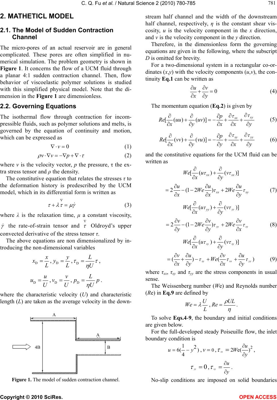

C. Q. Fu et al. / Natural Science 2 (2010) 780-785

781

2. MATHETICL MODEL

2.1. The Model of Sudden Contraction

Channel

The micro-pores of an actual reservoir are in general

complicated. These pores are often simplified in nu-

merical simulation. The problem geometry is shown in

Figure 1. It concerns the flow of a UCM fluid through

a planar 4:1 sudden contraction channel. Then, flow

behavior of viscoelastic polymer solutions is studied

with this simplified physical model. Note that the di-

mension in the Figure 1 are dimensionless.

2.2. Governing Equations

The isothermal flow through contraction for incom-

pressible fluids, such as polymer solutions and melts, is

governed by the equation of continuity and motion,

which can be expressed as

0v  (1)

vv p





  (2)

where v is the velocity vector, p the pressure, τ the ex-

tra stress tensor and ρ the density.

The constitutive equation that relates the stresses τ to

the deformation history is predescribed by the UCM

model, which in its differential form is written as



 





 (3)

where λ is the relaxation time, μ a constant viscosity,



 the rate-of-strain tensor and





Oldroyd’s upper

convected derivative of the stress tensor τ.

The above equations are non dimensionalized by in-

troducing the non-dimensional variables

,D





,

,D



.

where the characteristic velocity (U) and characteristic

length (L) are taken as the average velocity in the down-

B4B

Figure 1. The model of sudden contraction channel.

stream half channel and the width of the downstream

half channel, respectively, η is the constant shear vis-

cosity, u is the velocity component in the x direction,

and v is the velocity component in the y direction.

Therefore, in the dimensionless form the governing

equations are given in the following, where the subscript

D is omitted for brevity.

For a two-dimensional system in a rectangular co-or -

dinates (x,y) with the velocity components (u,v), the con-

tinuity Eq.1 can be written as







 (4)

The momentum equation (Eq.2) is given by

[() ()]

Re uuuv

yxxy





 







(5)

[() ()]

yyy

Re vvvu

yyxy





 







(6)

and the constitutive equations for the UCM fluid can be

written as

[()( )]

xxx

We uv









2(12 )2

xxy

uuu

We We





 



(7)

[()( )]

We uv









2(12 )2

yy xy

vvv

We We

yyx





 



(8)

[()( )]

xy xy

We uv









() ()

xyxx yy

vuv u

xyx y



 

 

 (9)

where τxx, τxy and τyy are the stress components in usual

sense.

The Weissenberg number (We) and Reynolds number

(Re) in Eq.9 are defined by

We L



,UL





.

To solve Eqs.4-9, the boundary and initial conditions

are given below.

For the full-developed steady Poiseuille flow, the inlet

boundary condition is

6( )

uy,0v



2e( )





,





,xy





.

No-slip conditions are imposed on solid boundaries

C. Q. Fu et al. / Natural Science 2 (2010) 780-785

782

and symmetry conditions are specified on the symmetri-

cal axis [9].

At the outlet a fully developed velocity profile is im-

posed with the homogeneous Neumann boundary condi-

tions for the extra-stress, i.e.,

xx xyyy

xxx









3. NUMERICAL ALGORITHM

The constitutive relation Eq . 3 is solved together with

Eqs.1 and 2 using the FVM. Here some details about our

own implementation of the method are given.

3.1. Computational Grid

A grid is placed in the computational domain and a

control volume is associated with each unknown on

the grid. This grid, called the reference grid, remains

fixed in space for all time. In this study, we assume

that the sides of each control volume are aligned with

the coordinate axes. Each component is integrated over

an appropriate control volume [10]. The grid is shown

in Figure 2.

The staggered grid is used in which the different de-

pendent variables are approximated at different mesh

points. Both meshes ensure that the solution is not pol-

luted by spurious pressure modes. On a non-staggered

mesh the familiar chequerboard mode is applied.

3.2. Discretization

A simple finite volume formulation is used for the dis-

cretization and the first-order Euler implicit formula is

used for temporal differences because of its simplicity

for implementation and unconditional stability in nu-

merical computations.

In employing the FVM, the governing equations are

written in the following general form [11]:

()( )mv S



  (10)

Figure 2. Staggered grid.

3.2.1. Discretization of Continuity Equations

The discretized continuity equation reflects the mass

conservation for each cell:

ewns

0FF FF



 (11)

where

FuyRe





, ww

FReuy,

FReux





, ss

FReux.

Fe is the outgoing mass flow rates at cell face e, ue refers

to the cell face velocity component, and the same for Fw,

Fn, Fs and uw , un , us.

3.2.2. Discretization of Momentum Equations

Eqs.5 and 6 can be written in the general form of Eq.10

using the transformation

xx xx

 



 (12)

yy yy

 





 (13)

()

xy xy





 



(14)

where





is the elastic part of the stress tensor



[12].

Substituting Eqs. 11-13 into the momentum equations

and assuming a constant viscosity turn Eqs.5 and 6 into

(Re) (Re)() ()

uu uv

yxxyy









()

xx uv p

yxxyx











 

 





(15)

(Re) (Re)()()

vv vu

yxxyy









 

()

yy xyuv p

yxxxyy









 

 





(16)

In Eqs.15 and 16 the viscous parts are discretized as

the diffusion terms of Eq.10, while the other terms on

the right-hand side are treated as extra source terms.

Then the final discretized equations of momentum can

be expressed symbolically in a general form:

PPEEWWNN SS u

auauaua uauS





(17)

where uP refers to the cell velocity component, and the

same for uE, uW, uN and uS.

max(, 0)





 ,

max(, 0)





 ,

Δxp

Δyp

P ue EE

uee

S SE

(δx)e

(δy)e vn vne

C. Q. Fu et al. / Natural Science 2 (2010) 780-785

783

max(, 0)







max(,0)





 .

3.2.3. Discretization of Constitutive Equations

The adopted viscoelastic model also has the general

transport equation from Eq.10 without diffusion term

(= 0). To ensure numerical stability, generally, a first-

order upwind difference (UD) is used for spatial discre-

tization. Thus, the discretized constitutive equation can

be written as

PPEEWWNN SSiijijijijijij

aaa aaS

 



 

  (18)

where τijP refers to the cell stress component, and the

same for τijE, τijW, τijN and τijS.

max(, 0)aWe F





, Ww

max( ,0)aWeF



,

max(,0)aWe F



, Ss

max(, 0)aWeF



,

PEWNS

axyaaaa



 

 

(2 )()

XX xx

SWeuuy



 

ns ns

2()( )

Weu uxv v





ns ns

(1)()( )

xy yy xy

SWeuuWevv



  

ew ew

()(1)()

xy xx

Weu uWev v



 

ew ew

2()2()

yy xy

SuuWevv



 

(2 )()

3yy

Wev v





where ve refers to the cell face velocity component, and

the same for vw, vn, vs.

3.3. Solution of the Discretized Equations

In non-linear problems the equations are solved with itera-

tive methods using an initial guess for the primitive vari-

ables and giving an approximate solution. The iterative

methods have the advantage of less computer memory as

they take advantage of zero elements in the coefficient

matrix. In this work, the strongly implicit procedure (SIP)

[13-15] is used, which involves the direct, simultaneous

solution of the set of equations formed by modification of

the original matrix equation. The modified matrix is con-

structed according to two criteria: 1) the equation set must

remain more strongly implicit than in the alternating direc-

tion implicit (ADI) case; and 2) the elimination procedure

for the modified set must be efficient.

4. RESULTS AND DISCUSSION

As discussed above, a numerical simulation method is

used and the stream function contour, velocity contour

and pressure contour with different We can be obtained.

As an example, the stream function and velocity con-

tours with We equates 0 to 3.0 are shown in Figures 3-5,

respectively.

(a) We = 0, Re = 10-5

(b) We = 0.6, Re = 10-5

(d) We = 3.0, Re = 10-5

Figure 3. Stream function contours.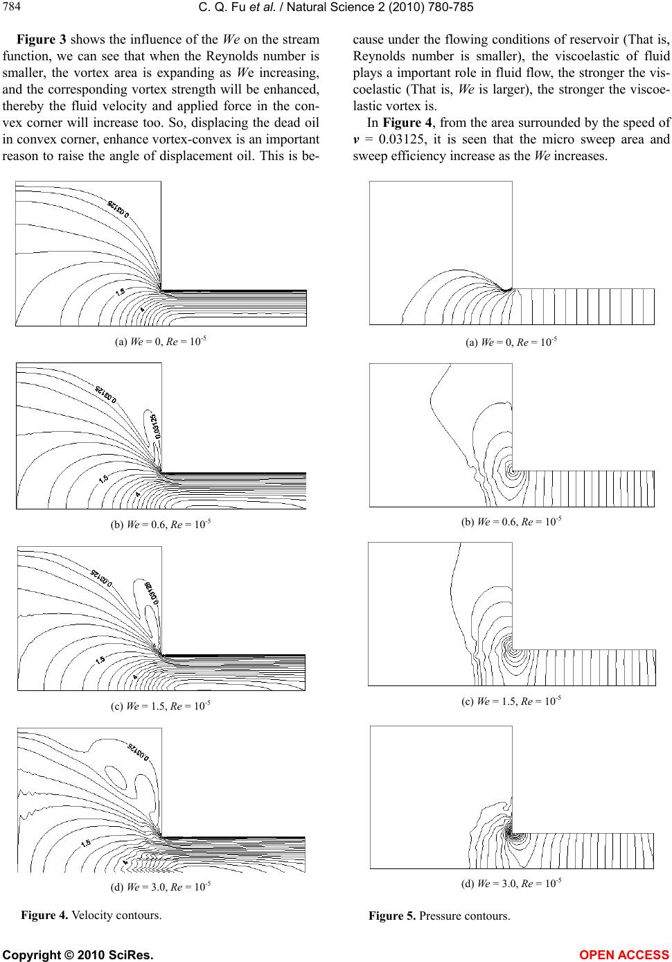

C. Q. Fu et al. / Natural Science 2 (2010) 780-785

784

Figure 3 shows the influence of the We on the stream

function, we can see that when the Reynolds number is

smaller, the vortex area is expanding as We increasing,

and the corresponding vortex strength will be enhanced,

thereby the fluid velocity and applied force in the con-

vex corner will increase too. So, displacing the dead oil

in convex corner, enhance vortex-convex is an important

reason to raise the angle of displacement oil. This is be-

(a) We = 0, Re = 10-5

(b) We = 0.6, Re = 10-5

(d) We = 3.0, Re = 10-5

Figure 4. Velocity contours.

cause under the flowing conditions of reservoir (That is,

Reynolds number is smaller), the viscoelastic of fluid

plays a important role in fluid flow, the stronger the vis-

coelastic (That is, We is larger), the stronger the viscoe-

lastic vortex is.

In Figure 4, from the area surrounded by the speed of

v = 0.03125, it is seen that the micro sweep area and

sweep efficiency increase as the We increases.

(a) We = 0, Re = 10-5

(b) We = 0.6, Re = 10-5

(d) We = 3.0, Re = 10-5

Figure 5. Pressure contours.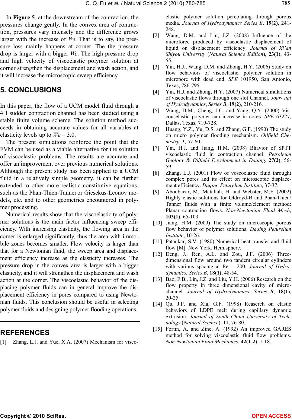

C. Q. Fu et al. / Natural Science 2 (2010) 780-785

785

In Figure 5, at the downstream of the contraction, the

pressures change gently. In the convex area of contrac-

tion, pressures vary intensely and the difference grows

larger with the increase of We. That is to say, the pres-

sure loss mainly happens at corner. The the pressure

drop is larger with a bigger We. The high pressure drop

and high velocity of viscoelastic polymer solution at

corner strengthen the displacement and wash action, and

it will increase the microscopic sweep efficiency.

5. CONCLUSIONS

In this paper, the flow of a UCM model fluid through a

4:1 sudden contraction channel has been studied using a

stable finite volume scheme. The solution method suc-

ceeds in obtaining accurate values for all variables at

elasticity levels up to We = 3.0.

The present simulations reinforce the point that the

FVM can be used as a viable alternative for the solution

of viscoelastic problems. The results are accurate and

offer an improvement over previous numerical solutions.

Although the present study has been applied to a UCM

fluid in a relatively simple geometry, it can be further

extended to other more realistic constitutive equations,

such as the Phan-Thien-Tanner or Giesekus-Leonov mo-

dels, etc. and to other geometries encountered in poly-

mer processing.

Numerical results show that the viscoelasticity of poly-

mer solutions is the main factor influencing sweep effi-

ciency. With increasing elasticity, the flowing area in the

corner is enlarged significantly, thus the area with immo-

bile zones becomes smaller. Flow velocity is larger than

that for a Newtonian fluid, the sweep area and displace-

ment efficiency increase as the elasticity increases. The

pressure drop in the convex area is larger with a bigger

elasticity, and it will strengthen the displacement and wash

action at the corner. The viscoelastic behavior of the dis-

placing polymer fluids can in general improve the dis-

placement efficiency in pores compared to using Newto-

nian fluids. This conclusion should be useful in selecting

polymer fluids and designing polymer flooding operations.

REFERENCES

[1] Zhang, L.J. and Yue, X.A. (2007) Mechanism for visco-

elastic polymer solution percolating through porous

media. Journal of Hydrodynamics Series B, 19(2), 241-

248.

[2] Wang, D.M. and Lin, J.Z. (2008) Influence of the

microforce produced by viscoelastic displacement of

liquid on displacement efficiency. Journal of Xi’an

Shiyou University (Natural Science Edition), 23(1), 43-

55.

[3] Yin, H.J., Wang, D.M. and Zhong, H.Y. (2006) Study on

flow behaviors of viscoelastic. polymer solution in

micropore with dead end. SPE 101950, San Antonio,

Texas, 786-795.

[4] Yin, H.J. and Zhong, H.Y. (2007) Numerical simulations

of viscoelastic flows through one slot Channel. Jour- nal

of Hydrodynamics, Series B, 19(2), 210-216.

[5] Wang, D.M., Cheng, J.C. and Yang, Q.Y. (2000) Vis-

couselastic polymer can increase in cores. SPE 63227,

Dallas, Texas, 719-728.

[6] Huang, Y.Z., Yu, D.S. and Zhang, G.F. (1990) The study

on micro polymer flooding mechanism. Oilfield Che-

mistry, 3, 57-60.

[7] Yin, H.J. and Jiang, H.M. (2008) Bhavior of SPTT

viscoelastic fluid in contraction channel. Petroleum

Geology & Oilfield Development in Daqing, 27(2), 56-

59.

[8] Zhang, L.J. (2001) Flow of voscoelastic fluid throught

complex pores and its effect on microscopic displace-

ment efficiency. Daqing Peturelum Institute, 37-37.

[9] Aboubacar, M., Matallah, H. and Webster, M.F. (2002)

Highly elastic solutions for Oldroyd-B and Phan-Thien/

Tanner fluids with a finite volume/element method:

Planar contraction flows. Non-Newtonian Fluid Mech,

103(1), 65-103.

[10] Jiang, H.M. (2009) The study on microscopic porous

flow behavior of polymer solutions. Daqing Peturelum

Institute, 10-26.

[11] Patankar, S.V. (1980) Numerical heat transfer and fluid

flow [M]. New York, Hemisphere.

[12] Deng, J., Ren, A.L. and Zou, J.F. (2006) Three-

dimensional flow around two tandem circular cylinders

with various spacing at Re = 200. Journal of Hydro-

dynamics, Series B, 18(1), 48-54.

[13] Bao, F.B., Lin, J.Z. and Liu, Y.H. (2006) Research on the

flow property in three dimensional cavity of micro-

channel. Journal of Hydrodynamics, Series B, 18(1),

20-25.

[14] Qu, J.P. and Xia, G.F. (1998) Reaserch on elastic

behaviors of LDPE melt during capillary dynamic

extrusion. Journal of South China University of Tech-

nology (Natural Science), 11, 76-80.

[15] Fortin, A. and Zine, A. (1992) An improved GARES

method for solving viscoelastic fluid flow problems.

Non-Newtonian Fluid Mechanics, 42(1-2), 1-18.