Study on Factors Effecting Weld Pool Geometry of Pulsed Current Micro Plasma Arc Welded AISI 304L Austenitic Stainless Steel Sheets Using Statistical Approach

Paper Menu >>

Journal Menu >>

Journal of Minerals and Materials Characterization and Engineering, 2012, 11, 790-799

Published Online August 2012 (http://www.SciRP.org/journal/jmmce)

Study on Factors Effecting Weld Pool Geometry of Pulsed

Current Micro Plasma Arc Welded AISI 304L Austenitic

Stainless Steel Sheets Using Statistical Approach

Kondapalli Siva Prasad1*, Chalamalasetti Srinivasa Rao2, Damera Nageswara Rao3

1Department of Mechanical Engineering, Anil Neerukonda Institute of Technology & Sciences, Visakhapatnam, India

2Department of Mechanical Engineering, Andhra University, Visakhapatnam, India

3Centurion University of Technology & Management, Odisha, India

Email: *[email protected]

Received March 27, 2012; revised May 5, 2012; accepted June 2, 2012

ABSTRACT

Pulsed current Mic ro Plas ma Arc W elding is used to joint thin sheets of AISI 304L sheets, which are used in manufac-

turing of metallic bellows and diaphragms. In this article the effects of pulsing current parameters on weld pool geome-

try namely front width, back width, front height and back height of pulsed current micro plasma arc welded AISI 304L

stainless steel sheets was analyzed. Four factors, five levels, central composite design was used to develop mathematical

models, incorporating pulsed current parameters and weld pool geometry. The mathematical models have been devel-

oped by Response Surface Method. The ad equacy of the models was checke d by ANOVA technique. Variation of out-

put responses with input process variables are discussed. By using the developed mathematical models, weld pool ge-

ometry parameters can be predicted.

Keywords: Pulsed Current; Micro Plasma Arc Welding; Mathematical Model; AIS I 304l St ai nl ess St eel ; Weld Poo l

Geometry; ANOVA

1. Introduction

Austenitic Chromium-Nickel stainless steels had gath-

ered wide acceptance in the fabrication of components

which require high temperature resistance and corrosion

resistance [1], such as metallic bellows used for fabrica-

tion of expa nsion joints, which are used in aircraft, aero-

space and petroleum industry, in which they are sub-

jected to high temperature and corrosive environment.

The present paper focuses on bellow manufacturing in

which a thin sheet is to fold round in shape an d the edges

has to be weld e d longitudinally.

The plasma welding process was introduced to the

welding industry in 1964 as a method of bringing better

control to the arc welding process in lower current ranges

[2]. Today, plasma retains the original advantages it

brought to the indu stry b y provid ing an adv anced lev el of

control and accuracy to produce high quality welds in

both miniature and pre precision applications and to pro-

vide long electrode life for high production requirements

at all levels of amperage. Plasma welding is equally

suited to manual and automatic applications. It is used in

a variety of joining operations ranging from welding of

miniature components to seam welding to high volume

production welding and many others.

Pulsed current MPAW involves cycling the welding

current at selected regular frequency. The maximum

current is selected to give adequate penetration and bead

contour, while the minimum is set at a level sufficient to

maintain a stable arc [3,4]. This permits arc energy to be

used effectively to fuse a spot of controlled dimensions

in a short time produ cing the weld as a series of overlap-

ping nuggets. By contrast, in constant welding current,

the heat required to melt the base material is supplied

only during the peak current pulses allowing the heat to

dissipate into the base material leading to narrower Heat

Affected Zone (HAZ). Advantages include improved

bead contours, greater tolerance to heat sink variations,

lower heat input requirements reduced residual stresses

and distortion, refinement of fusion zone microstructure

and reduced width of HAZ.

From the literature review [5-12] it was understood

that many researchers studied the influence of plasma arc

welding process parameters on bead geometry using sta-

tistical techniques like Taguchi, Response Surface Tech-

nique, Artificial Neural Network, Genetic Algorithm.

However in all the works reported so far researchers have

concentrated on materials of higher thickness; but not

*Corresponding author.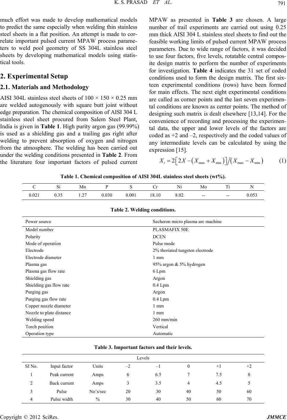

K. S. PRASAD ET AL. 791

much effort was made to develop mathematical models

to predict the same especially when welding thin stainless

steel sheets in a flat position. An attempt is made to cor-

relate important pulsed current MPAW process parame-

ters to weld pool geometry of SS 304L stainless steel

sheets by developing mathematical models using statis-

tical tools.

2. Experimental Setup

2.1. Materials and Methodology

AISI 304L stainless steel sheets of 100 × 150 × 0.25 mm

are welded autogenously with square butt joint without

edge preparation. The chemical composition of AISI 304 L

stainless steel sheet procured from Salem Steel Plant,

India is given in Table 1. High purity argon gas (99.99%)

is used as a shielding gas and a trailing gas right after

welding to prevent absorption of oxygen and nitrogen

from the atmosphere. The welding has been carried out

under the welding conditions presented in Table 2. From

the literature four important factors of pulsed current

MPAW as presented in Table 3 are chosen. A large

number of trail experiments are carried out using 0.25

mm thick AISI 304 L stainless steel sheets to find out the

feasible working limits of pulsed current MPAW process

parameters. Due to wide range of factors, it was decided

to use four factors, five levels, rotatable central compos-

ite design matrix to perform the number of experiments

for investigation. Table 4 indicates the 31 set of coded

conditions used to form the design matrix. The first six-

teen experimental conditions (rows) have been formed

for main effects. The next eight experimental conditions

are called as corner points and the last seven experimen-

tal conditions are known as center points. The method of

designing such matrix is dealt elsewher e [13,14]. For the

convenience of recording and processing the experimen-

tal data, the upper and lower levels of the factors are

coded as +2 and –2, respectively and the coded values of

any intermediate levels can be calculated by using the

expression [15].



 

maxminmax min

XXXXXX



 



(1)

Table 1. Chemical composition of AISI 304L stainless steel sheets (wt%).

C Si Mn P S Cr Ni Mo Ti N

0.021 0.35 1.27 0.030 0.001 18.10 8.02 -- -- 0.053

Table 2. Welding conditions.

Power source Secheron micro plasma arc machine

Model number PLASMAFIX 50E

Polarity DCEN

Mode of operation Pulse mode

Electrode 2% thoriated tungsten electrode

Electrode diameter 1 mm

Plasma gas 95% argon & 5% hydr o g e n

Plasma gas flow rate 6 Lpm

Shielding gas Argon

Shielding gas flow rate 0.4 Lpm

Purging gas Argon

Purging gas flow rat e 0.4 Lpm

Copper nozzle diameter 1 mm

Nozzle to plate distance 1 mm

Welding speed 260 mm/min

Torch position Vertical

Operation type Automatic

Table 3. Important factors and their levels.

Levels

SI No. Input factor Units –2 –1 0 +1 +2

1 Peak current Amps 6 6.5 7 7.5 8

2 Back current Amps 3 3.5 4 4.5 5

3 Pulse No’s/sec 20 30 40 50 60

4 Pulse width % 30 40 50 60 70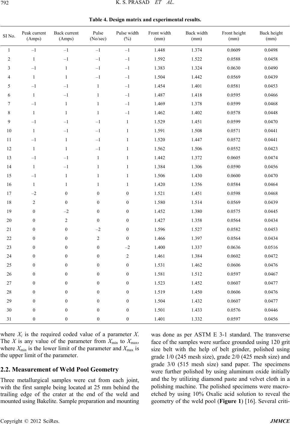

K. S. PRASAD ET AL.

792

Table 4. Design matrix and experimental results.

SI No. Peak current

(Amps) Back current

(Amps) Pulse

(No/sec) Pulse width

(%) Front width

(mm) Back width

(mm) Front height

(mm) Back height

(mm)

1 –1 –1 –1 –1 1.448 1.374 0.0609 0.0498

2 1 –1 –1 –1 1.592 1.522 0.0588 0.0458

3 –1 1 –1 –1 1.383 1.324 0.0630 0.0490

4 1 1 –1 –1 1.504 1.442 0.0569 0.0439

5 –1 –1 1 –1 1.454 1.401 0.0581 0.0453

6 1 –1 1 –1 1.487 1.418 0.0595 0.0466

7 –1 1 1 –1 1.469 1.378 0.0599 0.0468

8 1 1 1 –1 1.462 1.402 0.0578 0.0448

9 –1 –1 –1 1 1.529 1.451 0.0599 0.0470

10 1 –1 –1 1 1.591 1.508 0.0571 0.0441

11 –1 1 –1 1 1.520 1.447 0.0572 0.0441

12 1 1 –1 1 1.562 1.506 0.0552 0.0423

13 –1 –1 1 1 1.442 1.372 0.0605 0.0474

14 1 –1 1 1 1.384 1.306 0.0590 0.0456

15 –1 1 1 1 1.506 1.430 0.0600 0.0470

16 1 1 1 1 1.420 1.356 0.0584 0.0464

17 –2 0 0 0 1.521 1.451 0.0598 0.0468

18 2 0 0 0 1.580 1.514 0.0569 0.0439

19 0 –2 0 0 1.452 1.380 0.0575 0.0445

20 0 2 0 0 1.427 1.358 0.0564 0.0434

21 0 0 –2 0 1.596 1.527 0.0582 0.0453

22 0 0 2 0 1.466 1.397 0.0564 0.0434

23 0 0 0 –2 1.400 1.337 0.0636 0.0516

24 0 0 0 2 1.461 1.384 0.0602 0.0472

25 0 0 0 0 1.531 1.462 0.0606 0.0476

26 0 0 0 0 1.581 1.512 0.0597 0.0467

27 0 0 0 0 1.523 1.452 0.0607 0.0477

28 0 0 0 0 1.519 1.450 0.0606 0.0476

29 0 0 0 0 1.504 1.432 0.0607 0.0477

30 0 0 0 0 1.501 1.433 0.0576 0.0446

31 0 0 0 0 1.401 1.332 0.0597 0.0456

where Xi is the required coded value of a parameter X.

The X is any value of the parameter from Xmin to Xmax,

where Xmin is the lower limit of the parameter and Xmax is

the upper limit of the parameter.

2.2. Measurement of Weld Pool Geometry

Three metallurgical samples were cut from each joint,

with the first sample being located at 25 mm behind the

trailing edge of the crater at the end of the weld and

mounted using Bakelite. Sample preparation and mounting

was done as per ASTM E 3-1 standard. The transverse

face of the samples were surface grounded using 120 grit

size belt with the help of belt grinder, polished using

grade 1/0 (245 mesh size), grade 2/0 (425 mesh size) and

grade 3/0 (515 mesh size) sand paper. The specimens

were further polished by using aluminum oxide initially

and the by utilizing diamond paste and velvet cloth in a

polishing machine. The polished specimens were macro-

etched by using 10% Oxalic acid solution to reveal the

geometry of the weld pool (Figure 1) [16]. Several criti-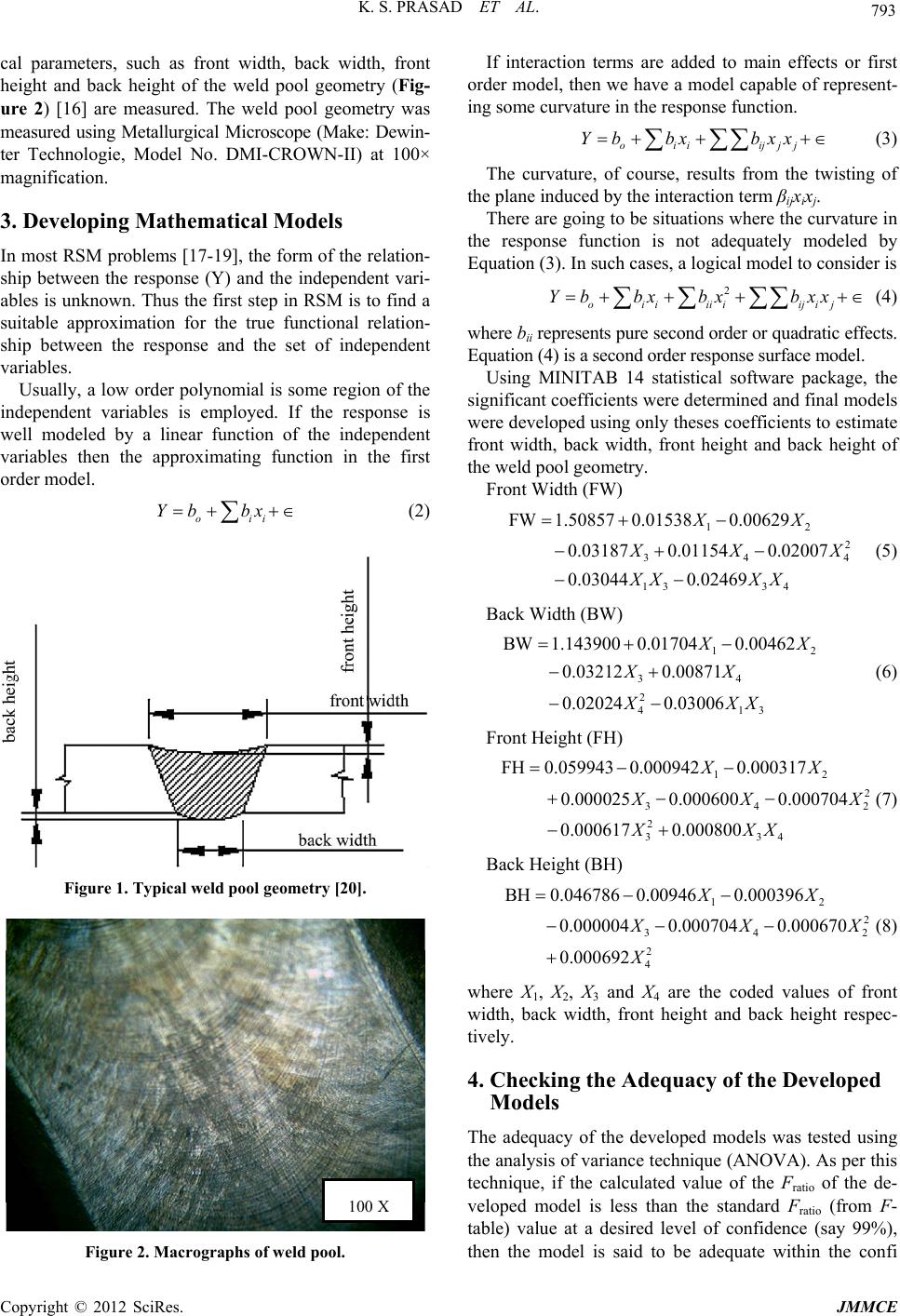

K. S. PRASAD ET AL. 793

cal parameters, such as front width, back width, front

height and back height of the weld pool geometry (Fig-

ure 2) [16] are measured. The weld pool geometry was

measured using Metallurgical Microscope (Make: Dewin-

ter Technologie, Model No. DMI-CROWN-II) at 100×

magnification.

3. Developing Mathematical Models

In most RSM problems [17-19], the form of the relation-

ship between the response (Y) and the independent vari-

ables is unknown. Thus the first step in RSM is to find a

suitable approximation for the true functional relation-

ship between the response and the set of independent

variables.

Usually, a low order polynomial is some region of the

independent variables is employed. If the response is

well modeled by a linear function of the independent

variables then the approximating function in the first

order model.

oii

bx Yb



(2)

Figure 1. Typical weld pool geometry [20].

100 X

o iiijjj

Yb bxbxx

Figure 2. Macrographs of weld pool.

If interaction terms are added to main effects or first

order model, then we have a model capable of represent-

ing some curvature in the response function.



 





oiiiii ijij

Ybbx bxbxx

(3)

The curvature, of course, results from the twisting of

the plane induced by th e interaction term βijxixj.

There are going to be situations where the curvature in

the response function is not adequately modeled by

Equation (3). In such cases, a logical model to consider is



 





344

13 34

FW1.50857 0.015380.00629

0.031870.011540.02007

0.030440.02469

(4)

where bii represents pure second order or quadratic effects.

Equation (4) is a second order response surface model.

Using MINITAB 14 statistical software package, the

significant coefficients were determined and final models

were developed using only theses coefficients to estimate

front width, back width, front height and back height of

the weld poo l geo metry.

Front Widt h ( FW)

XX XX

 





413

BW1.143900 0.017040.00462

0.032120.00871

0.020240.03006

(5)

Back Width (BW)

XXX









342

334

FH0.059943 0.0009420.000317

0.0000250.0006000.000704

0.0006170.000800

(6)

Front Height (FH)

XXX

 





342

BH0.046786 0.009460.000396

0.0000040.0007040.000670

0.000692

(7)

Back Heig h t (BH)

 





(8)

where X1, X2, X3 and X4 are the coded values of front

width, back width, front height and back height respec-

tively.

4. Checking the Adequacy of the Developed

Models

The adequacy of the developed models was tested using

the analysis of variance technique (ANOVA). As per this

technique, if the calculated value of the Fratio of the de-

veloped model is less than the standard Fratio (from F-

table) value at a desired level of confidence (say 99%),

then the model is said to be adequate within the confi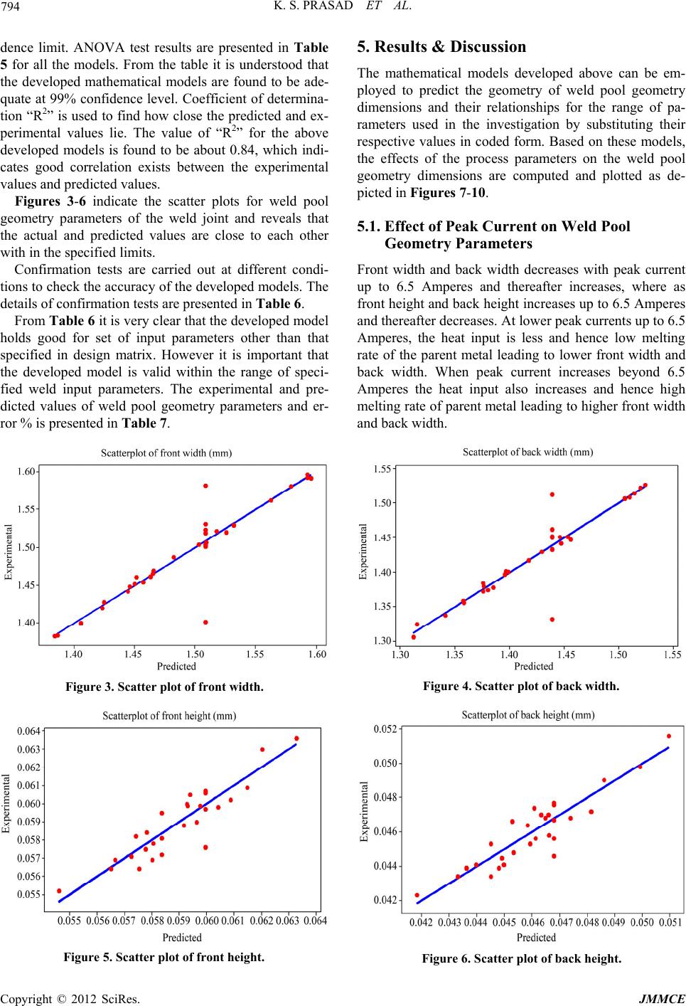

K. S. PRASAD ET AL.

JMMCE

794

5. Results & Discussion

dence limit. ANOVA test results are presented in Table

5 for all the models. From the table it is understood that

the developed mathematical models are found to be ade-

quate at 99% confidence level. Coefficient of determina-

tion “R2” is used to find how close the predicted and ex-

perimental values lie. The value of “R2” for the above

developed models is found to be about 0.84, which indi-

cates good correlation exists between the experimental

values and predicte d values.

The mathematical models developed above can be em-

ployed to predict the geometry of weld pool geometry

dimensions and their relationships for the range of pa-

rameters used in the investigation by substituting their

respective values in coded form. Based on these models,

the effects of the process parameters on the weld pool

geometry dimensions are computed and plotted as de-

picted in Figures 7-10.

Figures 3-6 indicate the scatter plots for weld pool

geometry parameters of the weld joint and reveals that

the actual and predicted values are close to each other

with in the specified limits.

5.1. Effect of Peak Current on Weld Pool

Geometry Parameters

Confirmation tests are carried out at different condi-

tions to check the accuracy of the developed models. The

details of confirmation tests are presented in Table 6.

Front width and back width decreases with peak current

up to 6.5 Amperes and thereafter increases, where as

front height and back height increases up to 6.5 Amperes

and thereafter decreases. At lower peak currents up to 6.5

Amperes, the heat input is less and hence low melting

rate of the parent metal leading to lower front width and

back width. When peak current increases beyond 6.5

Amperes the heat input also increases and hence high

melting rate of paren t metal leading to higher front width

and back width.

From Table 6 it is very clear that the developed model

holds good for set of input parameters other than that

specified in design matrix. However it is important that

the developed model is valid within the range of speci-

fied weld input parameters. The experimental and pre-

dicted values of weld pool geometry parameters and er-

ror % is presented in Table 7.

Figure 4. Scatter plot of back width.

Figure 3. Scatter plot of front width.

Figure 6. Scatter plot of back height.

Figure 5. Scatter plot of front height.

K. S. PRASAD ET AL. 795

Table 5. ANOVA table.

Front Width

Source DF Seq SS Adj SS Adj MS F P

Regression 14 0.100167 0.100167 0.007155 6.36 0.000

Linear 4 0.034205 0.034205 0.008551 7.60 0.001

Square 4 0.025671 0.025671 0.006418 5.70 0.005

Interaction 6 0.040291 0.040291 0.006715 5.96 0.002

Residual Error 16 0.018013 0.018013 0 .001126

Lack-of-Fit 10 0.000298 0.000298 0.000030 0.01 1.000

Pure Error 6 0.017716 0.017716 0.002953

Total 30 0.118180

Back Width

Source DF Seq SS Adj SS Adj MS F P

Regression 14 0.098374 0.098374 0.007027 6.18 0.000

Linear 4 0.034072 0.034072 0.008518 7.49 0.001

Square 4 0.026461 0.026461 0.006615 5.82 0.004

Interaction 6 0.037841 0.037841 0.006307 5.55 0.003

Residual Error 16 0.018191 0.018191 0 .001137

Lack-of-Fit 10 0.000509 0.000509 0.000051 0.02 1.000

Pure Error 6 0.017682 0.017682 0.002947

Total 30 0.116565

Front Height

Source DF Seq SS Adj SS Adj MS F P

Regression 14 0.000092 0.000092 0.000007 5.43

0.001

Linear 4 0.000032 0.000032 0.000008 6.71 0.002

Square 4 0.000038 0.000038 0.000009 7.85 0.001

Interaction 6 0.000021 0.000021 0.000004 2.97 0.038

Residual Error 16 0.000019 0.000019 0 .000001

Lack-of-Fit 10 0.000012 0.000012 0.000001 0.92 0.570

Pure Error 6 0.000008 0.000008 0.000001

Total 30 0.000111

Back Height

Source DF Seq SS Adj SS Adj MS F P

Regression 14 0.000102 0.000102 0.000007 5.54 0.001

Linear 4 0.000037 0.000037 0.000009 7.05 0.002

Square 4 0.000041 0.000041 0.000010 7.87 0.001

Interaction 6 0.000024 0.000024 0.000004 2.99 0.037

Residual Error 16 0.000021 0.000021 0 .000001

Lack-of-Fit 10 0.000012 0.000012 0.000001 0.78 0.656

Pure Error 6 0.000009 0.000009 0.000002

Total 30 0.000123

Where SS = sum of squares; M S = mean square s; DF = degree of freedom; F = fis her’s ratio.

K. S. PRASAD ET AL.

796

Table 6. Confirmation test results.

Weld pool geometry parameters (mm)

Experimental Predicted

Peak

current

(Amperes)

Back

current

(Amperes)

Pulse rate

(pulses/

second)

Pulse

width

(%) Front

Width Back

Width Front

Height Back

Height Front

Width Back

Width Front

Height Back

Height

2 2 2 2 1.1921.2460.0560.0341.1851.234 0.054 0.029

0 2 2 2 1.2801.3200.0620.0521.2761.311 0.056 0.048

2 0 2 2 1.2041.2320.0640.0381.1981.225 0.058 0.033

2 2 0 2 1.4761.4240.0560.0301.4701.410 0.053 0.026

Table 7. Comparison of experimental and predicte d value s.

Front width (mm) Back width (mm) Front height (mm) B a c k h e ig h t ( mm)

No. Experimental Predicted Error

(%) Experimental PredictedError

(%)

1 1.448 1.446 0.138 1.374 1.380 –0.4350.0609 0.0615–0.9760.0498 0.0499 –0.200

2 1.592 1.593 –0.063 1.522 1.519 0.1970.0588 0.0592–0.6760.0458 0.0466 –1.717

3 1.383 1.384 –0.072 1.324 1.315 0.6840.0630 0.06201.6130.0490 0.0486 0.823

4 1.504 1.503 0.067 1.442 1.447 –0.3460.0569 0.0580–1.8970.0439 0.0448 –2.009

5 1.454 1.457 –0.206 1.401 1.399 0.1430.0581 0.0584–0.5140.0453 0.0459 –1.307

6 1.487 1.482 0.337 1.418 1.418 0.0000.0595 0.05841.8840.0466 0.0453 2.870

7 1.469 1.465 0.273 1.378 1.385 –0.5050.0599 0.05980.1670.0468 0.0465 0.645

8 1.462 1.463 –0.068 1.402 1.396 0.4300.0578 0.0580–0.3450.0448 0.0453 –1.104

9 1.529 1.532 –0.196 1.451 1.453 –0.1380.0599 0.0593 1.0120.0470 0.0466 0.858

10 1.591 1.596 –0.313 1.508 1.510 –0.1320.0571 0.0573–0.3490.0441 0.0440 0.227

11 1.520 1.526 –0.393 1.447 1.456 –0.6180.0572 0.0584–2.0550.0441 0.0450 –2.000

12 1.562 1.562 0.000 1.506 1.505 0.0660.0552 0.05461.0990.0423 0.0418 1.196

13 1.442 1.444 –0.139 1.372 1.375 –0.2180.0605 0.0594 1.8520.0474 0.0461 2.820

14 1.384 1.387 –0.216 1.306 1.312 –0.4570.0590 0.0596–1.0070.0456 0.0461 –1.085

15 1.506 1.509 –0.199 1.430 1.429 0.0700.0600 0.05931.1800.0470 0.0463 1.512

16 1.420 1.423 –0.211 1.356 1.358 –0.1470.0584 0.0578 1.0380.0464 0.0458 1.310

17 1.521 1.518 0.198 1.451 1.446 0.3460.0598 0.0604–0.9930.0468 0.0474 –1.266

18 1.580 1.579 0.063 1.514 1.514 0.0000.0569 0.05660.5300.0439 0.0436 0.688

19 1.452 1.450 0.138 1.380 1.376 0.2910.0575 0.0578–0.5190.0445 0.0449 –0.891

20 1.427 1.425 0.140 1.358 1.357 0.0740.0564 0.0565–0.1770.0434 0.0433 0.231

21 1.596 1.593 0.188 1.527 1.524 0.1970.0582 0.05741.3940.0453 0.0445 1.798

22 1.466 1.465 0.068 1.397 1.395 0.1430.0564 0.0575–1.9130.0434 0.0445 –2.472

23 1.400 1.405 –0.356 1.337 1.341 –0.2980.0636 0.0633 0.4740.0516 0.0510 1.176

24 1.461 1.451 0.689 1.384 1.375 0.6550.0602 0.0609–1.1490.0472 0.0481 –1.871

25 1.531 1.509 1.458 1.462 1.439 1.5980.0606 0.05991.1690.0476 0.0468 1.709

26 1.581 1.509 4.771 1.512 1.439 5.0730.0597 0.0599–0.3340.0467 0.0468 –0.214

27 1.523 1.509 0.928 1.452 1.439 0.9030.0607 0.05991.3360.0477 0.0468 1.923

28 1.519 1.509 0.663 1.450 1.439 0.7640.0606 0.05991.1690.0476 0.0468 1.709

29 1.504 1.509 –0.331 1.432 1.439 –0.4860.0607 0.0599 1.3360.0477 0.0468 1.923

30 1.501 1.509 –0.530 1.433 1.439 –0.4170.0576 0.0599–3.8400.0446 0.0468 –4.701

31 1.401 1.509 –7.157 1.332 1.439 –7.4360.0597 0.0599–0.3340.0456 0.0468 –2.564

K. S. PRASAD ET AL. 797

Figure 7. Main effects for front width.

Figure 8. Main effects for back width.

Figure 9. Main effects for front height.

K. S. PRASAD ET AL.

798

Figure 10. Main effe cts for back he i g ht.

5.2. Effect of Back Current on Weld Pool

Geometry Parameters reason for effect of pulse width on weld pool geometry

parameters is same as that of pulse rate. From 30% to

50% pulse width, the interval between pulse widths is

high and hence the heat input which enters the system at

a moment increases thereby increasing the front width

and back width. When the pulse width increase beyond

50% heat input which enters the system at a moment

decreases thereby decreasing the front width and back

width.

Front width, back width, front height increases up to 4

Amperes and thereafter decreases, where as back height

increases up to 3.5 Amperes and thereafter decreases. As

the back current is helpful in maintaining continuous arc

during welding, when the back current is low i.e. up to 4

Amperes, front width, back width and front height in-

creases due to higher and dominating peak current which

generates large amount of heat. When the back current is

increased beyond 4 Amperes, it balances the heat input

leading to lower heat input and hence front width, back

width and front height decreases.

From Figures 3-6, it was understood that a peak cur-

rent of 6.5 Amperes, back current of 3.5 Amperes, pulse

rate of 40 pulses/sec and pulse width of about 40% is

found to produce opti mum resu lts.

6. Conclusion

5.3. Effect of Pulse Rate on Weld Pool Geometry

Parameters A five level, four factor full, factorial design matrix based

on the central composite rotatable design technique was

used for the develop ment of mathematical models to pre-

dict the weld pool geometry parameters for AISI 304 L

stainless sheets welded by pulsed current micro plasma

arc welding process. The prediction results using mathe-

matical models are very close to the experimental results.

Peak Current is the most dominating factor out of the

selected parameters, since as peak current increases heat

input increases leading to wider front and back widths

and narrow front and back heights. For a peak current of

6.5 Amperes, back current of 3.5 Amperes, pulse rate of

40 pulses/second and pulse width of 40% the optimal

weld pool geometry parameters can be achieved. The

mathematical models are developed considering only

four factors and five levels (peak current, back current,

pulse rate and pulse width). However one may consider

more number of factors and their levels to improve the

mathematical model.

Front width and back width decreases up to 50 pulses/

second and thereafter increases, where as front height

increases up to 40 pulses/second and thereafter decreases

and back height increases up to 30 pulses/second and

thereafter decreases. This may be due to difference in

heat input caused by variation of pulse rate. From 20 to

50 pulses/second, the interval between pulses is low and

hence the heat input which enters the system at a moment

decreases thereby decreasing the front width and back

width. When the pulse rate increase beyond 50 pulses/sec

heat input which en ters the system at a moment increases

thereby increasing the front width and back width.

5.4. Effect of Pulse Width on Weld Pool

Geometry Parameters

Front width and back width increases up to 50% and

thereafter decreases, where as front height and back

height decreases up to 60% and thereafter increases. The

K. S. PRASAD ET AL. 799

7. Acknowledgements

The authors would like to thank Shri. R. Gopla Krishnan,

Director, M/s Metallic Bellows (I) Pvt Ltd., Chennai for

his support to carry out experimentation work.

REFERENCES

[1] T. D. Clark, “Department of Mechanical Engineering,”

Mater’s Thesis, Brigham Young University, Provo, 2005.

[2] M. Balasubramanian, V. Jayabalan and V. Balasubrama-

nian, “Effect of Process Parameters of Pulsed Current

Tungsten Inert Gas Welding on Weld Pool Geometry of

Titanium Welds,” Acta Metallurgica Sinica (English Let-

ters), Vol. 23, No. 4, 2010, pp. 312-320.

[3] M. Balasubramanian, V. Jayabalan and V. Balasubrama-

nian, “Optimizing the Pulsed Current Gas Tungsten Arc

Welding Parameters,” Journal of Materials Science &

Technology, Vol. 22, No. 6, 2006, pp. 821-825.

[4] G. M. Reddy, A. A. Gokhale and K. P. Rao, “Weld Mi-

crostructure Refinement in a 1441 Grade Aluminium-

Lithium Alloy,” Journal of Materials Science, Vol. 32,

No. 5, 1997, pp. 4117-4126.

doi:10.1023/A:1018662126268

[5] D. K. Zhang and J. T. Niu, “Application of Artificial

Neural Network Modeling to Plasma Arc Welding of

Aluminum Alloys,” Journal of Advanced Metallurgical

Sciences, Vol. 13, No. 1, 2000, pp. 194-200.

[6] S.-C. Chi and L.-C. Hsu, “A Fuzzy Radial Basi s Function

Neural Network for Predicting Multiple Quality Charac-

teristics of Plasma Arc Welding,” Joint 9th IFSA World

Congress and 20th NAFIPS International Conference,

Vancouver, 25-28 July 2001, pp. 2807-2812.

[7] Y. F. Hsiao, Y. S. Tarng and W. J. Huang, “Optimization

of Plasma Arc Welding Parameters by Using the Taguchi

Method with the Grey Relational Analysis,” Journal of

Materials and Manufacturing Processes, Vol. 23, No. 1,

2007, pp. 51-58. doi:10.1080/10426910701524527

[8] K. Siva, N. Muragan and R. Logesh, “Optimization of

Weld Bead Geometry in Plasma Transferred Arc Hard-

facing Austenitic Stainless Steel Plates Using Genetic

Algorithm,” The International Journal of Advanced Manu-

facturing Technology, Vol. 41, No. 1-2, 2008, pp. 24-30.

doi:10.1007/s00170-008-1451-3

[9] A. K. Lakshinarayana, V. Balasubramanian, R. Varaha-

moorthy and S. Babu, “Predicted the Dilution of Plasma

Transferred Arc Hardfacing of Stellite on Carbon Steel

Using Response Surface Methodology,” Metals and Ma-

terials International, Vol. 14, No. 6, 2008, pp. 779-789.

doi:10.3365/met.mat.2008.12.779

[10] V. Balasubramanian, A. K. Lakshminarayanan, R. Vara-

hamoorthy and S. Babu, “Application of Response Sur-

face Methodolody to Prediction of Dilution in Plasma

Transferred Arc Hardfacing of Stainless Steel on Carbon

Steel,” International Journal of Iron and Steel Research,

Vol. 16, No. 1, 2009, pp. 44-53.

[11] E. Taban, A. Dhooge and E. Kaluc, “Plasma Arc Welding

of Modified 12% Cr Stainless Steel,” Materials and Ma-

nufacturing Processes, Vol. 24, No. 6, 2009, pp. 649-656.

doi:10.1080/10426910902769152

[12] N. Kahraman, M. Taskin, B. Gulenc and A. Durgutlu,

“An Investigation into the Effect of Welding Current on

the Plasma Arc Welding of Pure Titanium,” Kovove Ma-

ter, Vol. 48, No. 3, 2010, pp. 179-184.

[13] N. Srimath and N. Muragan, “Prediction and Optimiza-

tion of Weld Bead Geometry of Plasma Transferred Arc

Hardfacing Valve Seat Rings,” European Journal of Sci-

entific Research, Vol. 51, No. 2, 2011, pp. 285-298.

[14] D. C. Montgomery, “ Design and Analysis of Experiments,”

3rd Edition, John Wiley & Sons, New York, 1991.

[15] G. E. P. Box, W. H. Hunter and J. S. Hunter, “Statistics

for Experiments,” John Wiley & Sons, New York, 1978.

[16] J. Ravindra and R. S. Parmar, “Mathematical Model to

Predict Weld Bead Geometry for Flux Cored Arc Weld-

ing,” Journal of Metal Construction, Vol. 19, 1987, pp.

45-52.

[17] W. G. Cochran and G. M. Cox, “Experimental Designs,”

John Wiley & Sons Inc., London, 1957.

[18] T. B. Barker, “Quality by Experimental Design,” ASQC

Quality Press, Milkwakee, 1985.

[19] W. P. Gardiner and G. Gettinby, “Experimental Design

Techniques in Statistical Practice,” Horwood, Chichester,

1998.

[20] K. S. Prasad, Ch. S. Rao and D. N. Rao, “Prediction of

Weld Pool Geometry in Pulsed Current Micro Plasma

Arc Welding of SS304L Stainless Steel Sheets,” Interna-

tional Transaction Journal of Engineering Management

& Applied Sciences & Technologies, Vol. 2, No. 3, 2011,

pp. 325-336.