The Mathematical Model for Particle Suspension Flow through Porous Medium

doi:10.4236/gm.2012.23009

Paper Menu >>

Journal Menu >>

Geomaterials, 2012, 2, 57-62

http://dx.doi.org/10.4236/gm.2012.23009 Published Online July 2012 (http://www.SciRP.org/journal/gm)

The Mathematical Model for Particle Suspension Flow

through Porous Medium

Hooman Fallah, Hosein Barzegar Fathi, Hamed Mohammadi

Department of Petroleum Engineering, Firoozabad Branch, Islamic Azad University, Firoozabad, Iran

Email: [email protected]

Received May 12, 2012; revised June 14, 2012; accepted June 24, 2012

ABSTRACT

Transport of suspensions and emulsions in porous media occurs in numerous processes of environmental, chemical,

petroleum and civil engineering. In this work, a mass balance particle transport equation which includes filtration has

been developed. The steady-state transport equation is presented and the solution to the complete advective-dispersion

equation for particulate suspension flow has been derived for the case of a constant filter coefficient. This model in-

cludes transport parameters which are particle advective velocity, particle longitudinal dispersion coefficient and filter

coefficient. This work recommends to be investigated by particle longitudinal dispersion calculation from experimental

data, directly. Besides, the numerical model needs to be developed for general case of a transition filter coefficient.

Keywords: Particulate Suspension Flow; Filtration Theory; Filtration Coefficient; Transport; Porous Medium;

Mathematical Model

1. Introduction

The transport of particulate suspensions in porous me-

dium occurs in a variety of industrial and natural process

such as wastewater treatment, propagation of pollutants

in subsurface environment, fouling of membranes and

seawater injection in oil reservoirs. Flow of solid and

liquid particles with particle capture by the rock takes

place during injection of seawater and produced water in

oil fields.

Particle transport and retention are mostly important

for the environmental processes, where the particle con-

centration must not exceed a safety value, while the per-

meability changes is important for petroleum production

due to its effect on well productivity and injectivity [1].

The study of particle retention in porous medium can

be dated back to the work of Iwasaki [2] who proposed

the following basic empirical for deep bed hydrosol fil-

tration.







 (1)

where:



is the specific volume of deposited material

(particle retained concentration), is the fluid superfi-

cial velocity, is the particle suspended concentration

and



is called the filtration coefficient.

The must used approach for evaluating colloid migra-

tion, retention and detachment is solute transport mass

balance equation with th e sink term for particle retention

[3,4].



cUD







 



 (2)



det

cU k











 (3)

The term



in Equation (3) is called filtration coeffi-

cient. Equations (1) and (2) together with the formula for

coefficient



are called the classical filtration theory in

above refere n ces.

In the current work, a theoretical investigation of par-

ticulate suspension flow through porous media has been

done. The steady-state transport equation is presented

and the solution has been derived. The filtration coeffi-

cient



will be discussed as a dominant parameter in

the particle transport and retention through porous me-

dium.

2. Particulate Suspension Flow through

Porous Medium

2.1. Filtration Theory

When fluid containing particles reaches a porous medium,

the liquid and the solid phase in the suspension can be

separated, either by depositing in the pore or accumulat-

ing in front of the surface. This is similar to what hap-

pens in the filtration process. Then, the retention process

of particles when flowing through a porous media is

called Deep Bed Filtration [5]. Th e deep filtration occurs

because of several mechanisms: the contacting of parti-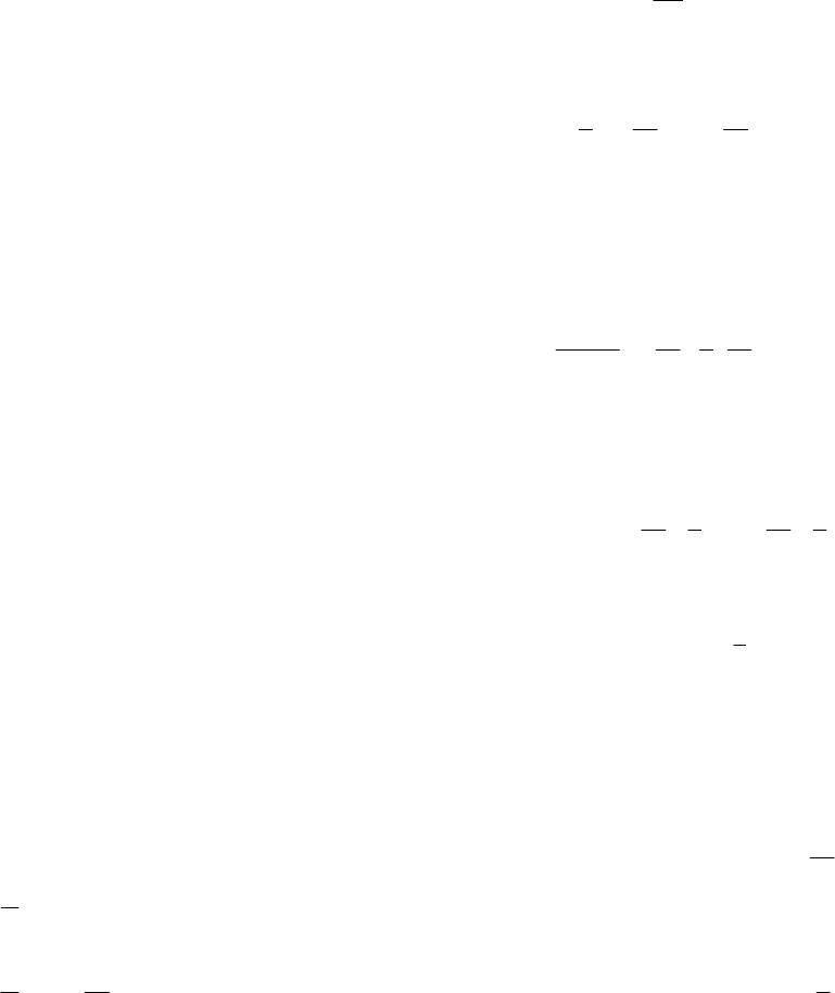

H. FALLAH ET AL.

cles with the retention site, the fixing of particle sites and

the breaking away of previously retained particles [6].

2.2. Mechanisms of Particles Retention

The particle capture in porous media can be caused by

different mechanisms [7].

• Size exclusion (large particles are captured in small

pores and pass through large p ores );

• Electrical forces (London-Van der Waals, double

electrical layer, etc.);

• Gravity segregation;

• Multi particle bridging.

3. Basic Formulation of Particles Transport

through Porous Medium

The model includes transport parameters which are parti-

cle advective velocity, particle longitudinal dispersion

coefficient and filter coefficient. These parameters have

been defined by dimensional analysis using the pertinent

variables of the porous medium system.

3.1. Advective Velocity

The averaged particle velocity in the porous media, has

been found to be either the same or slightly higher than

that of the carrier fluid. This deviation is caused by the

particle’s size. The expected difference can be deter-

mined by analyzing the velocity profiles of both the fluid

and the particles in a pore. The model has been formu-

lated for a capillary tube which has a constant rate with

the following assumption: No interactions between the

particles and the wall, suspension is well-mixed with a

constant concentration across the cross section .There is

no tran sverse flow.

(0 )rr













1

UU r







(0)

UU rr





 







 







rr a



 

(4)

As the particle travels through a tube, Brownian mo-

tion and shear action will cause the particle to travel

across the entire cross-section of the tube except that the

center-line of the particle will be excluded from the im-

mediate region of the wall due to its radial dimension.

After the particle has traveled far enough longitudi-

nally through the tube, the particle will have spent equal

amounts of time in all radial position across the capillary

tube. Integration of the velocity profile of Equation (4)

over the range of possible radii shown in Equation (4) for

both the particle and fluid yields the higher average ve-

locity for the particle than that for the carrier flu id.

The av erage flu i d velocity, in a capillary tube is:

V (5)

The average velocity of a particle,

V in a capillary

tube is:

VU rr























(6)

By inspecting Equation (5) and (6), the particles are

expected to have a larger average velocity than the car-

rier fluid velocity. This enhanced velocity of the particle

can be expressed as a fractional difference between the

two average velocities:

Soo

VVrr





 



(7)

This equation shows that as the radius of the particle

increase, the difference between the average particle ve-

locity and the average fluid interstitial velocity also in-

crease. This increase is not unbounded but reaches a

maximum



value for 3

r; as 3

r the

velocity difference decrease. In physical sense, the pore

radius can be estimated to approximately equal to

one-fifth of media grain diameter (1

rd); therefore

the largest possible particle to be able to fit through the

porous bed has a radius to this pore radius (

ar).



For a particle with



, the particles have been

shown to collect on the bed surface in a cake [6]. These

references show that the onset of deep bed filtration oc-

curs for a particle radius

a.less than

one-twentieth of the media grain diameter (1

ad

Particles with the radii larger than this will not transport

into the bed, but will collect on the surface. By lettingc



, the largest particle which will transport has a

radius equal t o one-fourth of the pore radius (1

ar).

3.2. Longitudinal Dispersion Coefficient

An important element of any dispersion model is the re-

presentation of the geometry of the porous medium.

Houseworth [8] has thoroughly reviewed such longitudi-

nal dispersion model for solute tracers. Instead of mod-

eling the internal structure of a porous medium, dimen-

sional analysis is used to analyze the problem. In this

study, the effect of mechanisms is expected to scale with

the pertinent transport variables.

The pertinent variables for solute dispersion are:

DL = longitudinal dispersion coefficient (L·T–1)

D = free fluid molecular diffusion coefficient of

H. FALLAH ET AL. 59

solute (L2·T–1)

Vs = fluid interstitial velocity (L·T–1)

and dg = media grain diameter (L)

From the Buckingham pi theorem, the following pairs

of groups are formed:

Vd D









ralternatively









D (8)

where Pec let nuPe mber Sg





Experimental data for solu te longitudinal dispersion in

uniform media show good correlation with these dimen-

sionless groups [8]. When the Peclet number is grater

than 1, the two groups can be re duced to one:

Constant

D

Vd (9)

where P

edynamic Peclet numbeSg





An order to magnitude approximation for the longitu-

dinal dispersion coefficient for solutes can be made with:

DdV



(10)

Particle longitudinal disp ersion is expected to be simi-

lar to that of solutes. Currently, no particle breakthro ughs

have been performed by others form which particle lon-

gitudinal dispersion coefficient be determined.

3.3. Filter Coefficient

Two approaches exist for analyzing the filter coefficient.

These are the macroscopic mass balance approach and

the microscopic trajectory analysis approach. Deep bed

filtration studies have been conducted to analyze both th e

system variables and the underlying mechanisms in-

volved in the processes of capturing and retaining parti-

cles in porous media .

3.3.1. Macros c opi c Approach

The macroscopic process of filtration or change in sus-

pension concentration over depth is first-order decay

with distance in steady flow. The filter coefficient may

be expressed as a function of single collector efficiency

and the single collector efficiency may be related to mi-

croscopic filtration mechanism.

Filtration results for steady state flow, neglecting lon-

gitudinal dispersion, gives:











(11)

C C expx



 

The filter coefficient theoretically may be expr essed as

the single collector efficiency as follows:















(12)

For T



, the particles under consideration are those

contained in a cylinder of diameter

d which is coinci-

dent with the vertical axis through the media grain col-

lector.



can be found either experimentally or from

the individual collector efficiency, T



and system vari-

ables using Equation (12).

The classical filtration theory assumes simultaneous

particle capture and dislodging. On the contrary, the

proposed model assumes that the particle capture takes

place only if the total of torques for electrostatic and

gravity forces prevails over the drag and lifting forces, so

the resulting torque presses the particle towards the ma-

trix or the internal cake.

3.3.2. Microscopic App roach

Microscopic study of particle motion near a collector is

defined as trajectory analysis. In porous media, particle

path far from media grains follow fluid streamline. As a

particle approach a media grain, the motion deviate from

the streamline because of various forces and torques act-

ing on the particles. These forces are presented by trans-

port and attachment mechanisms.

The transport mechanisms are: gravity settling, inter-

ception, Brownian diffusion and advection. The attach-

ment mechanisms are considered to be gravity, Lon-

don-van der Waals att racti on, do u bl e lay er fo rces.

From a combination of the trajectory analysis, the

three major contribution of filtration can be formulated.

These are collection due to Brownian diffusion, intercep-

tion and settling. Here, we assumed double layer repul-

sive forces and hydrodynamic retardation (slow drainage

of fluid from between two closely interacting particle

which occurs before contact of particles) are negligible.

The equations for these collection efficiencies are given

in the following [7].

Collection due t o Br ow ni an di ff usi o n,





 (13)

is constant. Also, either the particle Peclet number

can be allowed to reach a minimum value of approxi-

mately 1, or as 1



the efficiency reaches an as-

ymptotic value of 1.

Collection due to interception,

1.5



(14)





1.5 is constant here. Also the relative size group,



N, can be allowed to reach a minimum value of ap-

H. FALLAH ET AL.

proximately 1 in order for the efficiency to remain less

than or equal to 1.

As we mentioned before, the size of the largest parti-

cles which are able to penetrate and transport through a

porous bed is one twentieth of media grain diameter

da) or one-fourt h of the p ore radius (1

ar).

Collection due to settling,









TDIG



 (15)

The limit for this collection efficiency is the best pos-

sible collection which occurs for the settling velocity

equaling the interstitial velocity. As the settling velocity

becomes grater than the interstitial velocity, the effi-

ciency remains at a value of 1.

The equation for to tal collection efficiency is:







(16)

In this case,



has an asymptotic maximum value of

1. For Brownian particles (p), there is

good agreement between experimental and theoretical

result but for advective particles (p), it is

not, because of neglecting hydrodynamic retardation and

London-van der Waals attraction.

1.0dmicron

So, the exact analytical solution is [9]:

12 115

33 88

40.722.4 3

TSp SLORSGR

PeANNEAN N





 

(17)

The first term represents filtration due to Brownian

diffusion. The second and third terms represent the com-

bined effects of interception and gravity when the retar-

dation and London-van der Waals attraction are incl uded.

The effects of surface double layer forces are ignored

(attractive surface double layer is controlled by transport

processes and not depend on surface chemistry).

4. Modeling of Particle Transport and

Filtration

In this part, the steady-state transport equation is pre-

sented and the solution to the complete advective-dis-

persion equation for particulate suspension flow has been

derived for the case of a constant filter coefficient. This

model includes transport parameters which are particle

advestive velocity and particle longitudinal dispersion

coefficient. These parameters have been defined by di-

mensional analysis using the pertinent variables of the

porous media system.

4.1. Particle Advective Velocity

The result of the size exclusion for particles flowing in

capillary tube can be written as Equation (6) where



. By using the Equations (5), (6) and (7) we



will have:

1VV (18)





 (19)

As the particle size increase, the difference between

particle velocity and fluid velocity increase.

4.2. Particle Longitudinal Dispersion Coefficient

In modeling particle dispersion, the following variable

substitutions are used:

DD

VV

DD

Particle size variable can be removed by using the

particle properties as shown, provided 1

 also the

effect of particle size is included in the enhanced advec-

tive velocity for the particles.

This analysis shows that particle and solute longitudi-

nal dispersion are similar. When the particle Peclet

number (

Pe =

Pe D

 is grater than 10, the two

groups can be reduced to one :

constant

Vd  (20)

An order of magnitude approximation for the longitu-

dinal dispersion coefficient for particles can be made

with:

PPg

Vd

Pe 

10Pe 

(21)

As mentioned before, the dimensional argument for

defining the longitudinal dispersion coefficient is only

valid when . For uniform media, this restriction

is seen to be p. Flow conditions are simultane-

ously limited to the linear, laminar regime for which the

Reynolds number must be less than 10.

4.3. Steady-State Transport Equation and

Solution

Particle removal or filtration occurs as a particle suspen-

sion flows through a porous medium due to the interac-

tion of the advecting particles and grains of the medium.

Iwasaki [1] is credited with being the first to express fil-

tration a first-order decay of particle concentration with

distance:

H. FALLAH ET AL.

5. Conclusion









0Cx C



(22) In this work, a mass balance particle transport equation

which includes filtration has been d eveloped. This model

includes transport parameters which are particle advec-

tive velocity, particle longitudinal dispersion coefficient

and filter coefficient. The steady-state transport equation

is presented and the solution to the complete advective-

dispersion equation for particulate suspension flow has

been derived for the case of a constant filter coefficient.

(23)

and a solution in dimensional terms:



0expCC x





***

expCx



(24)

or in dimensionless terms:





 (25)



This work recommends to be investigated by particle

longitudinal dispersion calculation from experimental

data. Besides, the numerical model needs to be devel-

oped for general case of a transition filter coefficient.

where *







00CCx

6. Acknowledgements





The authors thank Professor P. Bedrikovetsky, Chair in

Petroleum Engineering, Australian School of Petroleum,

University of Adelaide.



A complete equation of steady-state filtration can be

formulated by using the general steady-state advection-

dispersion equation of transport for particle concentration

with a sink term to describe particle removal due to fil-

tration:

REFERENCES

[1] S. Pang and M. M. Sharma, “A Model for Predicting

Injectivity Decline in Water-Injection Wells,” SPE Paper

28489, Vol. 12, No. 3, 1997, pp. 194-201.

0LP

p p











0Cx C



lim 0

xCx

 





 (26) [2] T. Iwasaki, “Some Notes on Sand Filtration,” Water

Works Association, 1937, pp. 1591-1602,

The following semi-infinite medium boundary condi-

tions are: [3] J. W. A. Foppen and J. F. Schijven, “Evaluation of Data

from the Literature on the Transport and Survival of Es-

cherichia coil in Aquifers under Saturated Conditions,”

Journal of Water Research, Vol. 40, No. 3, 2006, pp.

401-426. doi:10.1016/j.watres.2005.11.018

(27) [4] J. F. Schijven and S. M. Hassanizadeh, “Removal of Vi-

ruses by Soil Passage: Overview of Modeling Processes,

and Parameters,” Critical Reviews in Environmental Sci-

ence and Technology, Vol. 30, No. 1, 2000, pp. 49-127

The solution which is shown in dimensional terms is

derived in appendix:





0expC xCx



 (28) [5] R. Farajzadeh, “An Experimental Investigation into In-

ternal Filtration and External Cake Build Up,” MSc. The-

sis, Delft University of Technology, 2004.

where 1114

PLP

LP P











[6] J. P. Herzig, D. M. Leclerc and P. Le Goff, “Flow of sus-

pension through porous media-application to deep filtra-

tion,” Journal of Industrial and Engineering Chemistry,

Vol. 65, No. 5, 1970, pp. 8-35

0Dp

***

*Dp

Pe C













**01Cx

(29)

[7] M. Elimelech and O’Melia, “Effect of Particle Size on

Collosion Efficiency in the Deposition of Brownian Par-

ticles with Electrostatic Barriers,” 1990, pp. 1153-1163

With the same boundary conditions:





m 0Cx

 

***

expCx



(30) [8] J. E. Houseworth, “Longitudinal Dispersion in Nonuni-

form, Isotropic Porous Media,” Ph.D. Thesis, W.M. Keck

Laboratory of Hydraulics and Water Resources, Califor-

nia Institute of Technology, Report No. KH-R-45, 1984.

x (31)

and a solution in dimensionless terms: [9] A.C. Paytakes and C. Tien, “Particle Deposition in Fi-

brous Media with Dendritic Pattern: Apreliminary

model,” Journal of Aerosol Science, Vol. 7, No. 2, 1976,

pp. 85-94. doi:10.1016/0021-8502(76)90067-7





 (32)

















dPe



 (33)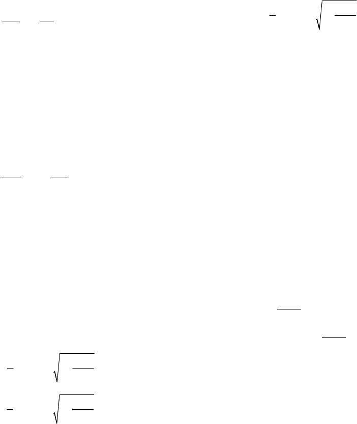

H. FALLAH ET AL.

Appendix. Solution Derivation

Consider the one-dimensional steady-state particle ad-

vective-dispersion equation which includes the removal

term to account for filtration effects:

0LP

P P











0Cx C



lim 0

xCx

 

 (A.1)

With the following boundary conditions:

(A.1.1)

For convenience, the x-variab le is allowed to range from

negative to positive infinity







 , although the

equation are only applied for x > 0 this avoids difficulty

at x = 0, because small dispersion is allowed. In dimen-

sionless form, the transport equ ation becomes:

0LP Dp

DPe

***

*Dp

PeC













**01Cx



m 0Cx

 

exp x



(A.2)

With the same boundary conditions:

x (A.2.1)

In order to derive a solution, try the following as a solu-

tion:













(A.3)

Check the equation (A.3) by substituting into Equation

(A.2), this results in second- deg ree po lyno mial in ter m of



and two roots of this polynomial are:











12DP















**** **

Bexp x









**01AB

 

B 

1and 0AB

12DP





Using these two roots, Equation (A.3) becomes:



C xAexpx





 (A.4)

The constants of this Equation can be determined by ap-

plying the boundary conditions:



Cx 



00A







By substituting these constants into Equation (A.4), the

solution to Equation (A.2) becomes:

** *

exp1 1

2DP

Cx Pex























(A.5)





Nomenclature

dg= media grain diameter (L)

dp= particle diameter (L)

c = suspended particle concentration in carrier fluid

σ = particle retained concentration

kdet = detachment rate coefficient

U = flow velocity

US = fluid velocity

UP = particle velocity

UO = fluid centerline velocity

r = radial distance

ro = capillary radius

ap = particle radius

p = dynamic pressure

x = longitudinal distance

DL = longitudinal dispersion coefficient (L·T–1)

D = free fluid molecular dispersion coefficient of solute

(L2·T–1)

VS = fluid interstitial velocity (L·T–1)

Pe = Peclet number = Sg

V.d

PeD = dynamic Pec let number = Sg

V.d

C = particle concentration (M·L–3)

X = longitudinal position (L)

λ = filter coefficient (L–1)

WS = particle settling velocity

VS = fluid interstitial velocity

Ρpf = densities of particle and fluid, respectively

g = gravitational acceleration

H = Hamakar constant (e r gs)

NG = gravitional group = ηG

DLP = particle longitudinal dispersion coefficient (L2·T–1)

DP = particle molecular diffusion coefficient in a free

fluid (L2·T–1)

VP = particle velocity (L2·T–1)