The Shortest Width Confidence Interval for Odds Ratio in Logistic Regression

doi:10.4236/ojs.2012.23037

Paper Menu >>

Journal Menu >>

Open Journal of Statistics, 2012, 2, 305-308

http://dx.doi.org/10.4236/ojs.2012.23037 Published Online July 2012 (http://www.SciRP.org/journal/ojs)

The Shortest Width Confidence Interval for Odds Ratio

in Logistic Regression

Eugene Demidenko

Section of Biostatistics and Epidemiology, Geisel School of Medicine at Dartmouth, Hanover, USA

Email: [email protected]

Received May 16, 2012; revised June 18, 2012; accepted July 2, 2012

ABSTRACT

The shortest width confidence interval (CI) for odds ratio (OR) in logistic regression is developed based on a theorem

proved by Dahiya and Guttman (1982). When the variance of the logistic regression coefficient estimate is small, the

shortest width CI is close to the regular Wald CI obtained by exponentiating the CI for the regression coefficient esti-

mate. However, when the variance increases, the optimal CI may be up to 25% narrower. It is demonstrated that the

shortest width CI is favorable because it has a smaller probability of covering the wrong OR value compared with the

standard CI. The closed-form iterations based on the Newton’s algorithm are provided, and the R function is supplied.

A simulation study confirms the superior properties of the new CI for OR in small sample. Our method is illustrated

with eight studies on parity as a preventive factor against bladder cancer in women.

Keywords: Bladder Cancer; Coverage Probability; Logistic Regression; Newton’s Algorithm





1/2 1/2

ˆˆ



1. Introduction

Odds ratio, as the exponentiated logistic regression co-

efficient, is a popular measure of association in medicine,

epidemiology and biostatistics. Routinely, the confidence

interval (CI) for odds ratio (OR) in logistic regression is

computed by exponentiating the CI for the beta-co-

efficient (log OR, hereafter denoted as



), [1,2]. While

it is true that if a CI for



has coverage probability



 the exponentiated CI for OR has the same

coverage probability, such CI does not have the shortest

width and therefore can be improved. The goal of this

note is to demonstrate how to compute the shortest CI for

OR using a theorem proved in [3]. Previously, [4] sug-

gested to find the shortest confidence interval for OR

using the same approach but their procedure of minimi-

zation of the interval’s width was just an approximate

solution. In this paper, we find the exact minimum via

Newton’s iterations.

2. The Method

Let the coefficient of logistic regression



be estimated

by maximum likelihood (ML) so that



ˆ,







OR =

large sample. We want to construct the shortest CI for



based on ˆ



assuming that its variance 2



is known. In practice, this variance is not known but

usually the sample size is large enough, so that one can

assume that 2



is fixed. Routinely, one first constructs

the CI for



100 1















 and then exponentiates it to ob-





100 1%



 CI for OR as tain the





1/2 1/2

ˆˆ









1/2





where is the







th

quantile of the standard normal cdf,





=12,z







=0.05

1/2



 where  is the cdf of the stand-

ard normal distribution. For example, if



have 1/2



 This CI will be refered to as the

(traditional) Wald CI with symmetric z-values.

=1.96.z

The idea of the shortest CI is to chose asymmetric

z-values such that the coverage probability is the same,





but the length of the CI is minimum. Thus we

seek CI for OR in the form





ˆˆ







<zz

(1)

where are such that









=1zz .



 

=zz

(2)





. Clearly, the standard CI has the form (1) with

Since the width of interval (1) is OR we





arrive at the following optimization problem:





min zz



 (3)

under restriction (2). As was shown by Dahiya and Guttman

(1982), this optimization problem reduces to the solution

of the following system of equations for z1 and z2: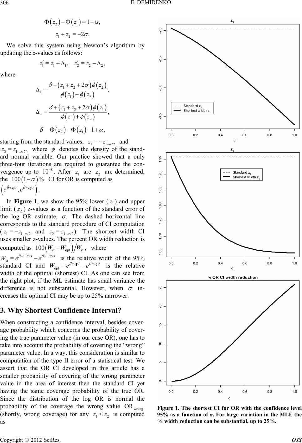

E. DEMIDENKO

306

 

=1 ,zz



 

=2.zz





2 22

= ,z z









We solve this system using Newton’s algorithm by

updating the z-values as follows:

11 1

=,zz



where



zz

2











zz

1













=1,zz







=zz

starting from the standard values, 11/2



 and

21/2



 where



=,zz



denotes the density of the stand-

ard normal variable. Our practice showed that a only

three-four iterations are required to guarantee the con-

vergence up to . After 1 are 2 are determined,

the CI for OR is computed as

8z10 z











%100

,ee







.

In Figure 1, we show the 95% lower (1) and upper

limit (2) z-values as a function of the standard error of

the log OR estimate, .



The dashed horizontal line

corresponds to the standard procedure of CI computation

(11/2

=zz





=).zz



and 21/2



 The shortest width CI

uses smaller z-values. The percent OR width reduction is

computed as st

ˆˆ

1.96 1.96

st =We e

optst ,WWW100 where













ˆˆ

=zz

is the relative width of the 95%

standard CI and opt







 is the relative

width of the optimal (shortest) CI. As one can see from

the right plot, if the ML estimate has small variance the

difference is not substantial. However, when



in-

creases the optimal CI may be up to 25% narrower.

3. Why Shortest Confidence Interval?

When constructing a confidence interval, besides cover-

age probability which concerns the probability of cover-

ing the true parameter value (in our case OR), one has to

take into account the probability of covering the “wrong”

parameter value. In a way, this consideration is similar to

computation of the type II error of a statistical test. We

assert that the OR CI developed in this article has a

smaller probability of covering of the wrong parameter

value in the area of interest then the standard CI yet

having the same coverage probability of the true OR.

Since the distribution of the log OR is normal the

probability of the coverage the wrong value wrong

(shortly, wrong coverage) for any is computed

<zz Figure 1. The shortest CI for OR with the confidence level

95% as a function of σ. For large variation in the MLE the

% width reduction c a n be substantial, up to 25%.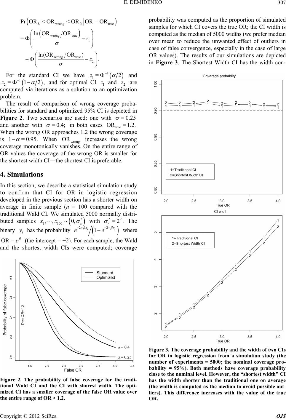

E. DEMIDENKO 307



wrong

wrong true

PrOR< OR< OR

ln OROR

ln(OROR )



















true

OR= OR













For the standard CI we have









1 and z



=12,





 z z

=0.25

2 and for optimal CI 1 and 2 are

computed via iterations as a solution to an optimization

problem.

The result of comparison of wrong coverage proba-

bilities for standard and optimized 95% CI is depicted in

Figure 2. Two scenarios are used: one with



and another with =0.4;



in both cases true

When the wrong OR approaches 1.2 the wrong coverage

OR= 1.2.

1= 0.95.



 When wrong increases the wrong

coverage monotonically vanishes. On the entire range of

OR values the coverage of the wrong OR is smaller for

the shortest width CI—the shortest CI is preferable.

100

4. Simulations

In this section, we describe a statistical simulation study

to confirm that CI for OR in logistic regression

developed in the previous section has a shorter width on

average in finite sample (n = 100 compared with the

traditional Wald CI. We simulated 5000 normally distri-

buted samples



~0,

1,,





with . The





binary has the probability 22







OR= e

 where



(the intercept = −2). For each sample, the Wald

and the shortest width CIs were computed; coverage

Figure 2. The probability of false coverage for the tradi-

tional Wald CI and the CI with shorest width. The opti-

mized CI has a smaller coverage of the false OR value over

the entire range of OR > 1.2.

probability was computed as the proportion of simulated

samples for which CI covers the true OR; the CI width is

computed as the median of 5000 widths (we prefer median

over mean to reduce the unwanted effect of outliers in

case of false convergence, especially in the case of large

OR values). The results of our simulations are depicted

in Figure 3. The Shortest Width CI has the width con-

Figure 3. The coverage probability and the width of two CIs

for OR in logistic regression from a simulation study (the

number of experiments = 5000; the nominal coverage pro-

bability = 95%). Both methods have coverage probability

close to the nominal level. However, the “shortest width” CI

has the width shorter than the traditional one on average

(the width is computed as the median to avoid possible out-

liers). This difference increases with the value of the true

R. O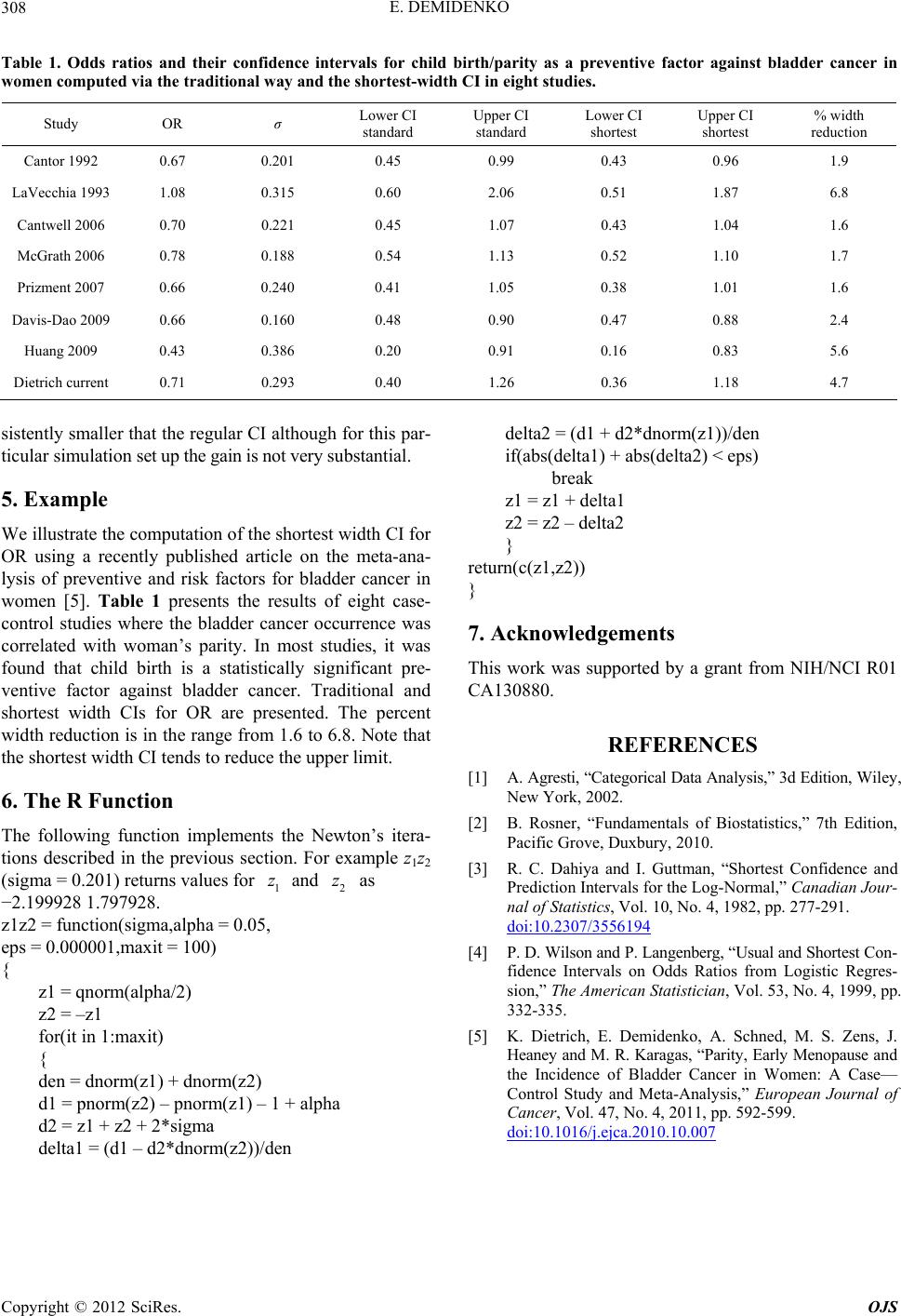

E. DEMIDENKO

308

Table 1. Odds ratios and their confidence intervals for child birth/parity as a preventive factor against bladder cancer in

women computed via the traditional way and the shortest-width CI in eight studies.

Study OR σ Lower CI

standard

Upper CI

standard

Lower CI

shortest

Upper CI

shortest

% width

reduction

Cantor 1992 0.67 0.201 0.45 0.99 0.43 0.96 1.9

LaVecchia 1993 1.08 0.315 0.60 2.06 0.51 1.87 6.8

Cantwell 2006 0.70 0.221 0.45 1.07 0.43 1.04 1.6

McGrath 2006 0.78 0.188 0.54 1.13 0.52 1.10 1.7

Prizment 2007 0.66 0.240 0.41 1.05 0.38 1.01 1.6

Davis-Dao 2009 0.66 0.160 0.48 0.90 0.47 0.88 2.4

Huang 2009 0.43 0.386 0.20 0.91 0.16 0.83 5.6

Dietrich current 0.71 0.293 0.40 1.26 0.36 1.18 4.7

delta2 = (d1 + d2*dnorm(z1))/den sistently smaller that the regular CI although for this par-

ticular simulation set up the gain is not very substantial. if(abs(delta1) + abs(delta2) < eps)

break

5. Example z1 = z1 + delta1

z2 = z2 – delta2

We illustrate the computation of the shortest width CI for

OR using a recently published article on the meta-ana-

lysis of preventive and risk factors for bladder cancer in

women [5]. Table 1 presents the results of eight case-

control studies where the bladder cancer occurrence was

correlated with woman’s parity. In most studies, it was

found that child birth is a statistically significant pre-

ventive factor against bladder cancer. Traditional and

shortest width CIs for OR are presented. The percent

width reduction is in the range from 1.6 to 6.8. Note that

the shortest width CI tends to reduce the upper limit.

}

return(c(z1,z2))

}

7. Acknowledgements

This work was supported by a grant from NIH/NCI R01

CA130880.

REFERENCES

[1] A. Agresti, “Categorical Data Analysis,” 3d Edition, Wiley,

New York, 2002.

6. The R Function

[2] B. Rosner, “Fundamentals of Biostatistics,” 7th Edition,

Pacific Grove, Duxbury, 2010.

The following function implements the Newton’s itera-

tions described in the previous section. For example z1z2

(sigma = 0.201) returns values for and as

−2.199928 1.797928.

[3] R. C. Dahiya and I. Guttman, “Shortest Confidence and

Prediction Intervals for the Log-Normal,” Canadian Jour-

nal of Statistics, Vol. 10, No. 4, 1982, pp. 277-291.

doi:10.2307/3556194

z1z2 = function(sigma,alpha = 0.05,

eps = 0.000001,maxit = 100) [4] P. D. Wilson and P. Langenberg, “Usual and Shortest Con-

fidence Intervals on Odds Ratios from Logistic Regres-

sion,” The American Statistician, Vol. 53, No. 4, 1999, pp.

332-335.

{

z1 = qnorm(alpha/2)

z2 = –z1

for(it in 1:maxit) [5] K. Dietrich, E. Demidenko, A. Schned, M. S. Zens, J.

Heaney and M. R. Karagas, “Parity, Early Menopause and

the Incidence of Bladder Cancer in Women: A Case—

Control Study and Meta-Analysis,” European Journal of

Cancer, Vol. 47, No. 4, 2011, pp. 592-599.

doi:10.1016/j.ejca.2010.10.007

{

den = dnorm(z1) + dnorm(z2)

d1 = pnorm(z2) – pnorm(z1) – 1 + alpha

d2 = z1 + z2 + 2*sigma

delta1 = (d1 – d2*dnorm(z2))/den