

Paper Menu >>
Journal Menu >>
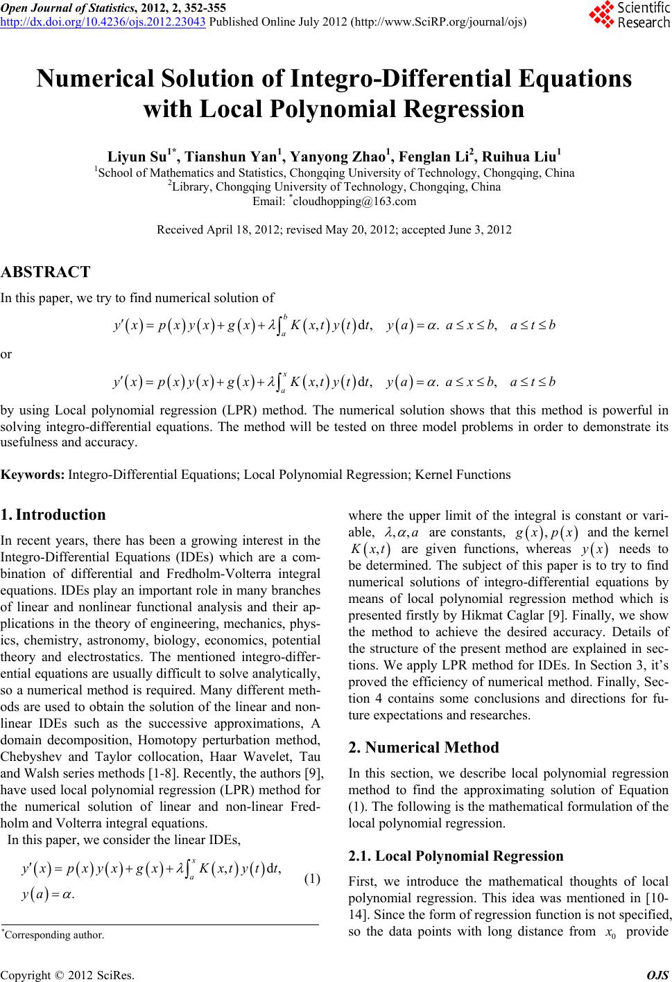 Open Journal of Statistics, 2012, 2, 352-355 http://dx.doi.org/10.4236/ojs.2012.23043 Published Online July 2012 (http://www.SciRP.org/journal/ojs) Numerical Solution of Integro-Differential Equations with Local Polynomial Regression Liyun Su1*, Tianshun Yan1, Yanyong Zhao1, Fenglan Li2, Ruihua Liu1 1School of Mathematics and Statistics, Chongqing University of Technology, Chongqing, China 2Library, Chongqing University of Technology, Chongqing, China Email: *[email protected] Received April 18, 2012; revised May 20, 2012; accepted June 3, 2012 ABSTRACT In this paper, we try to find numerical solution of b d, . a yxpxyxgxKxtyttyaax ba tb d,. , a yxpxyxgxKxtyttyaax ba tb dxtytt ya a or x by using Local polynomial regression (LPR) method. The numerical solution shows that this method is powerful in solving integro-differential equations. The method will be tested on three model problems in order to demonstrate its usefulness and accuracy. Keywords: Integro-Differential Equations; Local Polynomial Regression; Kernel Functions 1. Introduction In recent years, there has been a growing interest in the Integro-Differential Equations (IDEs) which are a com- bination of differential and Fredholm-Volterra integral equations. IDEs play an important role in many branches of linear and nonlinear functional analysis and their ap- plications in the theory of engineering, mechanics, phys- ics, chemistry, astronomy, biology, economics, potential theory and electrostatics. The mentioned integro-differ- ential equations are usually difficult to solve analytically, so a numerical method is required. Many different meth- ods are used to obtain the solution of the linear and non- linear IDEs such as the successive approximations, A domain decomposition, Homotopy perturbation method, Chebyshev and Taylor collocation, Haar Wavelet, Tau and Walsh series methods [1-8]. Recently, the authors [9], have used local polynomial regression (LPR) method for the numerical solution of linear and non-linear Fred- holm and Volterra integral equations. In this paper, we consider the linear IDEs, x a yxpxyx gxK (1) where the upper limit of the integral is constant or vari- able, are constants, g xpx and the kernel K xt y are given functions, whereas x 0 needs to be determined. The subject of this paper is to try to find numerical solutions of integro-differential equations by means of local polynomial regression method which is presented firstly by Hikmat Caglar [9]. Finally, we show the method to achieve the desired accuracy. Details of the structure of the present method are explained in sec- tions. We apply LPR method for IDEs. In Section 3, it’s proved the efficiency of numerical method. Finally, Sec- tion 4 contains some conclusions and directions for fu- ture expectations and researches. 2. Numerical Method In this section, we describe local polynomial regression method to find the approximating solution of Equation (1). The following is the mathematical formulation of the local polynomial regression. 2.1. Local Polynomial Regression First, we introduce the mathematical thoughts of local polynomial regression. This idea was mentioned in [10- 14]. Since the form of regression function is not specified, so the data points with long distance from x provide *Corresponding author. C opyright © 2012 SciRes. OJS 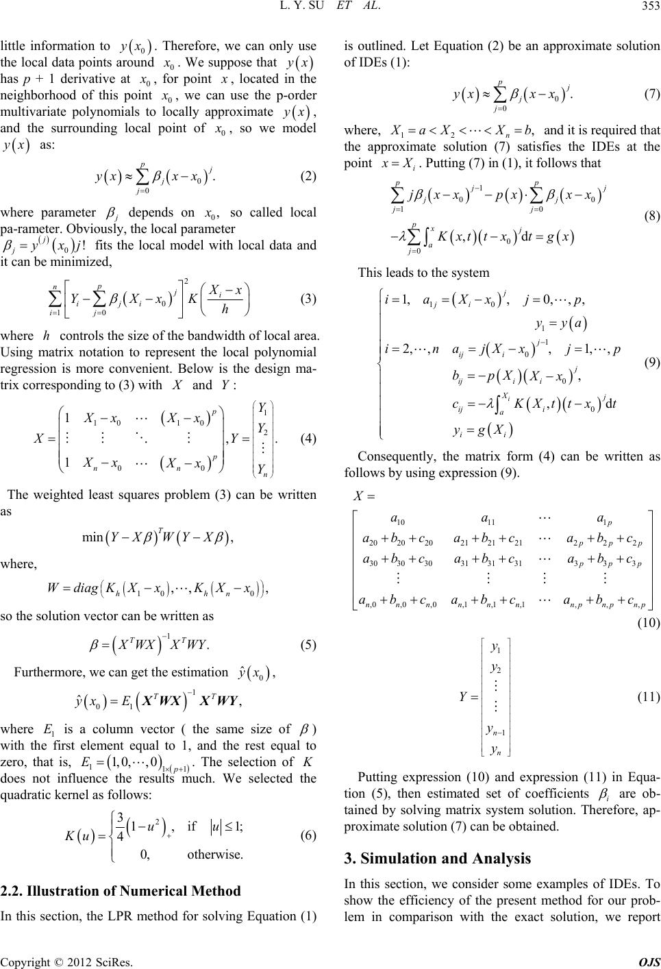 L. Y. SU ET AL. 353 little information to 0 y x. Therefore, we can only use the local data points around 0 x . We suppose that y x has p + 1 derivative at 0 x , for point x , located in the neighborhood of this point 0 x , we can use the p-order multivariate polynomials to locally approximate y x, and the surrounding local point of 0 x , so we model y x as: . 0 0 p j j j yx x x (2) where parameter j depends on 0 x so called local pa-rameter. Obviously, the local parameter j fits the local model with local data and it can be minimized, 0 j yx!j 2 0 j ij 10 p ij ni i X x h Y K Xx (3) where controls the size of the bandwidth of local area. Using matrix notation to represent the local polynomial regression is more convenient. Below is the design ma- trix corresponding to (3) with h X and Y: 10 00 p p x XY ,X 1 2 n Y Y Y WY 10 nn Xx X Xx Xx 1 1 . (4) min The weighted least squares problem (3) can be written as T YX 0 , n x 1T where, 10 K x hh KXWdiag X so the solution vector can be written as . T X WY 0 ˆ XW X (5) Furthermore, we can get the estimation y x 1, , yx 01 E ˆTT X WXX WY where 1 is a column vector ( the same size of E ) with the first element equal to 1, and the rest equal to zero, that is, 111p 10 0E . The selection of does not influence the results much. We selected the quadratic kernel as follows: K 2 3if 4 0otherwise u 1 1u Ku 0 0 . p (6) 2.2. Illustration of Numerical Method In this section, the LPR method for solving Equation (1) is outlined. Let Equation (2) be an approximate solution of IDEs (1): j j j yx x x (7) where, 12 n X aXX b i and it is required that the approximate solution (7) satisfies the IDEs at the point x X . Putting (7) in (1), it follows that 1 00 10 0 0 d pp j j jj jj pxj a j jpx x xxx Kxtt gxtx 10 1 1 0 0 0 1,,0,,, 2, ,,1,, , ,d i j ji j ij i j ijii Xj ij i a ii iaj pXx yya inaj jpXx bpX Xx cKXtttx ygX 10 111 2020 2021 21 21222 30 303031 3131333 000 111 p ppp ppp nnnn n nnpnpnp X aa a abc abcabc abc abcabc abcabc abc (8) This leads to the system (9) Consequently, the matrix form (4) can be written as follows by using expression (9). 1 2 1n n y y Y y y (10) (11) Putting expression (10) and expression (11) in Equa- tion (5), then estimated set of coefficients i are ob- tained by solving matrix system solution. Therefore, ap- proximate solution (7) can be obtained. 3. Simulation and Analysis In this section, we consider some examples of IDEs. To show the efficiency of the present method for our prob- lem in comparison with the exact solution, we report Copyright © 2012 SciRes. OJS 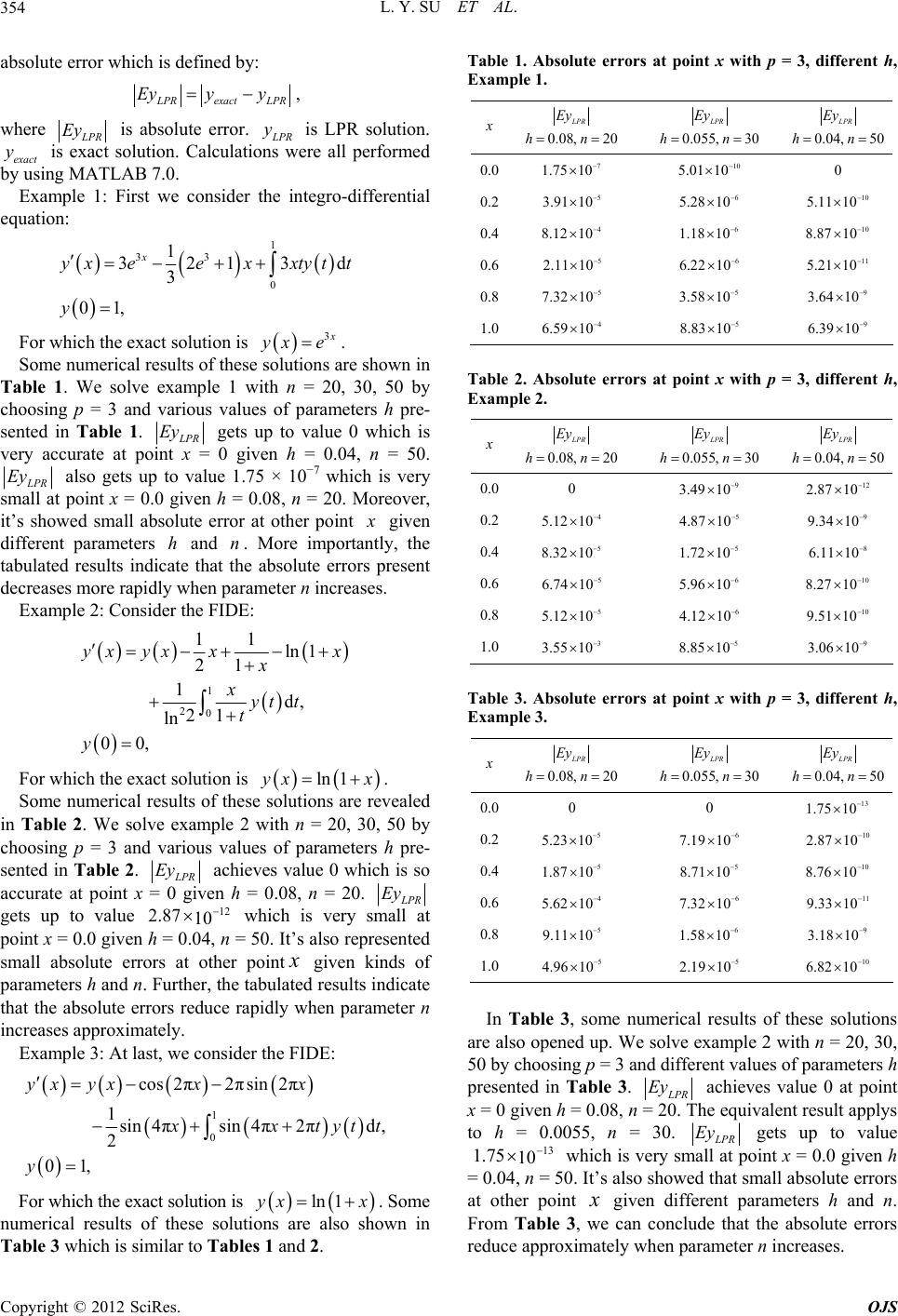 L. Y. SU ET AL. 354 absolute error which is defined by: L PR Ey exact LPR y y , where L PR is absolute error. Ey L PR is LPR solution. exact is exact solution. Calculations were all performed by using MATLAB 7.0. y y Example 1: First we consider the integro-differential equation: 1 33 0 1 321 3 01, x yx eex y 3dxtyt t 3 For which the exact solution is x yx e. Some numerical results of these solutions are shown in Table 1. We solve example 1 with n = 20, 30, 50 by choosing p = 3 and various values of parameters h pre- sented in Table 1. L PR gets up to value 0 which is very accurate at point x = 0 given h = 0.04, n = 50. Ey L PR also gets up to value 1.75 × 10⁻⁷ which is very small at point x = 0.0 given h = 0.08, n = 20. Moreover, it’s showed small absolute error at other point Ey x given different parameters and . More importantly, the tabulated results indicate that the absolute errors present decreases more rapidly when parameter n increases. hn Example 2: Consider the FIDE: ln 1 d 1 20 11 21 1 21 ln 00, y xyx x x t y x x yt t ln 1 For which the exact solution is y xx. Some numerical results of these solutions are revealed in Table 2. We solve example 2 with n = 20, 30, 50 by choosing p = 3 and various values of parameters h pre- sented in Table 2. L PR achieves value 0 which is so accurate at point x = 0 given h = 0.08, n = 20. Ey L PR gets up to value which is very small at point x = 0.0 given h = 0.04, n = 50. It’s also represented small absolute errors at other point Ey 12 287 10 x given kinds of parameters h and n. Further, the tabulated results indicate that the absolute errors reduce rapidly when parameter n increases approximately. Example 3: At last, we consider the FIDE: 1 0 cos 2π2πsin 2π 1sin 4πsin 4π2 2 01, yx yxx πd x x xtytt ln 1 y For which the exact solution is y Table 1. Absolute errors at point x with p = 3, different h, Example 1. xx. Some numerical results of these solutions are also shown in Table 3 which is similar to Tables 1 and 2. x 008, 20 LPR Ey hn 0 055,30 LPR Ey hn 004, 50 LPR Ey hn 0.0 7 175 10 10 501 10 0 0.2 5 391 10 6 52810 10 511 10 4 812 10 0.4 6 118 10 10 887 10 5 211 10 0.6 6 622 10 11 521 10 5 732 10 0.8 5 35810 9 364 10 4 659 10 1.0 5 883 10 9 639 10 Table 2. Absolute errors at point x with p = 3, different h, Example 2. x 008, 20 LPR Ey hn 0 055,30 LPR Ey hn 004, 50 LPR Ey hn 0.00 9 349 10 12 287 10 0.2 4 512 10 5 487 10 9 934 10 5 832 10 0.4 5 172 10 8 611 10 5 674 10 0.6 6 596 10 10 827 10 5 512 10 0.8 6 412 10 10 951 10 3 35510 1.0 5 88510 9 306 10 Table 3. Absolute errors at point x with p = 3, different h, Example 3. x 008, 20 LPR Ey hn 0 055,30 LPR Ey hn 004, 50 LPR Ey hn 0.00 0 13 175 10 0.2 5 52310 6 719 10 10 287 10 5 187 10 0.4 5 871 10 10 876 10 4 562 10 0.6 6 732 10 11 93310 5 911 10 0.8 6 158 10 9 31810 5 496 10 1.0 5 219 10 10 682 10 In Table 3, some numerical results of these solutions are also opened up. We solve example 2 with n = 20, 30, 50 by choosing p = 3 and different values of parameters h presented in Table 3. L PR achieves value 0 at point x = 0 given h = 0.08, n = 20. The equivalent result applys to h = 0.0055, n = 30. Ey L PR gets up to value Ey 13 175 10 which is very small at point x = 0.0 given h = 0.04, n = 50. It’s also showed that small absolute errors at other point x given different parameters h and n. From Table 3, we can conclude that the absolute errors reduce approximately when parameter n increases. Copyright © 2012 SciRes. OJS  L. Y. SU ET AL. Copyright © 2012 SciRes. OJS 355 4. Conclusion In this paper, we make use of LPR method to solve the linear integro-differential equations. It’s showed that this method is very convergent for solving linear integro-dif- ferential equations. Moreover, the numerical results ap- proximate the exact solution very well. The Method can be extended to different parameters p, h and kinds of kernel functions. LPR method can also solve nonlinear or integro-differential equations which can be researched and resolved. 5. Acknowledgements This work was in part supported by Chongqing CSTC foundations of China (Grant No. CSTC, 2010BB2310, Grant No. CSTC, 2011jjA40033), Chongqing CMEC foundations of China (Grant No. KJ080614, Grant No. KJ100810, Grant No. KJ100818, KJ120829). REFERENCES [1] B. Asady and M. T. Kajani, “Direct Method for Solving Integro Differential Equations Using Hybrid Fourier and Block-Pluse Functions,” International Journal of Com- puter Mathematics, Vol. 82, No. 7, 2007, pp. 889-895. doi:10.1080/00207160412331336044 [2] D. F. Han and X. F. Shang, “Numerical Solution of Inte- gro-Differential Equations by Using CAS Wavelet Op- erational Matrix of Integration,” Vol. 156, No. 2, Applied Mathematics Computation, 2007, pp. 460-466. doi:10.1016/j.amc.2007.04.048 [3] A. Golbabai and M. Javidi, “Application of He’s Homo- topy Perturbation Method for nth-Order Integro-Differen- tial Equations,” Applied Mathematics Computation, Vol. 190, No. 2, 2007, pp. 1409-1416. doi: 10.1016/j.amc.2007.02.018 [4] A. Karamete and M. Sezer, “A Taylor Collocation Method for the Solution of Linear Integro-Differential Equations,” International Journal of Computer Mathematics, Vol. 79, No. 9, 2002, pp. 987-1000. doi:10.1080/00207160216116 [5] H. Jaradat, O. Alsayyed and S. Al-Shara, “Numerical Solution of Linear Integro-Differential Equations 1,” Jour- nal of Mathematics Statistics, Vol. 4, No. 4, 2008, pp. 250-254. doi: 10.1.1.152.8509 [6] K. Maleknejad and F. Mizaee, “Numerical Solution of Integro-Differential Equations by Using Rationalized Haar Functions Method,” International Journal of System Ma- thematics, Vol. 35, No. 10, 2006, pp. 1735-1744. doi 10.1108/03684920610688694 [7] J. Pour-Mahmoud, M. Y. Rahimi-Ardabili and S. Shah- morad, “Numerical Solution of the System of Fredholm Integro-Differential Equations by the Tau Method,” Ap- plied Mathematics Computation, Vol. 168, No. 1, 2005, pp. 465-478. doi:10.1016/j.amc.2004.09.026 [8] M. T. Rashed, “Numerical Solution of Functional Differen- tial, Integral and Integro-Differential Equations,” Ap- plied Numerical Mathematics, Vol. 156, No. 2, 2004, pp. 485-492. doi:10.1016/j.amc.2003.08.021 [9] H. Caglar and N. Caglar, “Numerical Solution of Integral Equations by Using Local Polynomial Regression,” Jour- nal of Computational Analysis and Applications, Vol. 10, No. 2, 2008, pp. 187-195. [10] L. Y. Su, Y. Y. Zhao and T. S. Yan, “Two-Stage Method Based on Local Polynomial Fitting for a Linear Hetero- scedastic Regression Model and Its Application in Eco- nomics,” Discrete Dynamics in Nature and Society, Vol. 2012, 2012, Article ID 696927. doi:10.1155/2012/696927 [11] L. Y. Su, “Prediction of Multivariate Chaotic Time Series with Local Polynomial Fitting,” Computers Mathematics with Applications, Vol. 59, No. 2, 2010, pp. 737-744. doi:10.1016/j.camwa.2009.10.019 [12] L. Y. Su, Y. J. Ma and J. J. Li, “Application of Local Polynomial Estimation in Suppressing Strong Chaotic Noise,” Ch i n e se Physics B , 2012, Vol. 21, No. 2, 2012. doi:10.1088/1674-1056/21/2/020508 [13] J. Fan and I. Gijbels, “Local Polynomial Modelling and Its Applications, Vol. 66 of Monographs on Statistics and Applied Probability,” Chapman Hall, London, 1996. [14] J. Fan and Q. Yao, “Nonlinear Time Series: Nonparamet- ric and Parametric Methods, Springer Series in Statistics,” Springer, Berlin, 2003. |