The Threshold Effects of RMB Exchange Rate Fluctuations on Imports and Exports

doi:10.4236/jfrm.2012.12003

Paper Menu >>

Journal Menu >>

Journal of Financial Risk Management

2012. Vol.1, No.2, 15-20

Published Online June 2012 in SciRes (http://www.SciRP.org/journal/jfrm) http://dx.doi.org/10.4236/jfrm.2012.12003

The Threshold Effects of RMB Exchange Rate Fluctuations

on Imports and Exports

Chuanglian Chen

School of Economics and Management, South China Normal University, Guangzhou, China

Email: [email protected]

Received March 10th, 2012; revised April 27th, 2012; accepted May 18th, 2012

Using threshold panel model, we estimate the effectiveness of exchange rate to imports and exports. We

conclude that there is a second threshold in both import and export regression models, and China’s trade

flows don’t accord with ML condition, when RMB exchange rate appreciation is less than 7.8%. Whereas,

when higher than 7.8%, the ML condition strongly holds, indicating that the RMB exchange rate appre-

ciation would deteriorate the China’s international revenue. As RMB exchange rate to US dollar has ex-

periences an appreciation of 22.2% from 2005Q3 to 2012Q1, thus China’s current account would be dete-

riorated. Therefore, some changes or policies should be made to deal with these problems.

Keywords: Threshold Effects, Exchange Rate, Imports, Marshall-Lener Condition

Introduction

On July 21, 2005, the People’s Bank of China makes a deci-

sion that the exchange rate regime was changed from a de facto

peg to the US dollar to a more flexible peg to a basket of for-

eign currencies. And on April 16, 2012, the PBC relaxes ex-

change rate fluctuations bands to 1%. As to this, the RMB ex-

change rate to US dollar has experiences an appreciation of

22.2% from 2005Q3 to 2012Q1. According to the traditional

elasticity theory, the exchange rate appreciation will lower

exports and increase imports. Moreover, if the Marshall-Lerner

condition holds, exchange rate (domestic currency) apprecia-

tion would deteriorate international revenue and devaluation

will improve the net trade flows.

The elasticity approach is still the most commonly used in

balance of trade flows analysis. Recently, a large body of lite-

ratures has reexamined the impact of exchange rate fluctuations

on the balance of trade through examining the ML condition

from a theoretical point of view. Oskooee-Bahmani (1998) ,

Bahmani-Oskooee and Kara (2003), De Silva and Zhu(2004) et

al. find that most countries’ trade elasticities are large enough

to support devaluation as a successful policy for improving the

balance of trade flows. Whereas, Wilson (2001) concludes that

there is no J-curve for Malaysia, Korea and Singapore, and the

ML conditions is not met. Luis Sastre (2012) also supports this

conclusion for other countries.

As to most domestic studies, the related empirical studies can

be classified into three categories. First, Li Yining (1991) ar-

gues that the demand elasticities of imports and exports are

insufficient. Second, the elasticities of exchange rate to trade

flows only reaches the critical value, thus the effect of ex-

change rate fluctuations to China’s trade is relatively small

(Chen, 1992). Third, most recently empirical literatures show

that ML condition holds in China (Dai, 1997; Feng, 2007; Liu,

Zhou, & Xu, 2010).

Although the conclusions are different in the above studies,

but all of them use linear model as an application. As the im-

pacts of exchange rate variations on imports and exports may

be non-linear, therefore, we employ the threshold panel model,

proposed by Hansen (1996, 1999), to estimate the threshold

effects. And then, analyze different threshold effects of ex-

change rate variations to imports and exports. From the empiri-

cal conclusions, we not only can test the effective of exchange

rate appreciation on trade, but also examine how large the ex-

change rate can appreciation, and wouldn’t deteriorate trade

flows.

Theoretical Model and Threshold Panel

Regression Model

Theoretical Model

Following the recent literature, we assume that the main de-

terminants of a country’s exports and imports are income, rela-

tive prices and trade cost. Thus, we assume that exports and

import demand function for each country take the form of





,, ,,

EXEX YPXPXTE



 and IM = IM(Y, PM, PD, T, E),

where EX and IM stand for exports and imports, respectively.

Yis China’s income, and Y



is trade partners’ income. PM

stands for import price, PD stands for domestic price, T denotes

trade cost, E denotes exchange rate, PX is export price, PX



is trade partners’ export price. Consider PD = PX = P, where P

is domestic price. PM= PX* = P*, where P

* is trade foreign

partners’ domestic price.

In order to estimate the effect of exchange rate to imports

and exports, as ESPP





αβ δ λ

texext itext

exy te



 

αβ δλ

timimt itim

imy te 

, where S denotes the bilateral

nominal exchange rate. Following the literature, we assume that

the rest of the trade partners’ demand for a country’s exports

(ex) and imports (im) take the following log-form:

(1)

(2)

where, the lowercase letters represent the logarithmic form of

the corresponding capital letters. As for the model, domestic

currency (exchange rate) appreciation would increase imports if

C. L. CHEN

λ0

0δ0

β0

0

β0

im , and exchange rate appreciation would reduce exports

if ex . denotes that trade cost would reduce both

imports and export. im indicates that the improvement of

the domestic income would increase imports, however, if the

domestic income is increased by imports substitution, then

im . indicates that the improvement of the for-

eign trade partners’ income would increase exports, however, if

income is increased by exports substitution, then ex

β0βex



(Kara, 2002). Furthermore, the Marshall-Lener condition holds

if λλ

im ex

1



Threshold Panel Regression Model

In order to capture whether there is a structural change rela-

tionship between dependent variable and independent variables.

We use threshold panel regression model, proposed by Hansen

(1996, 1999), as an application. Consider a threshold panel

regression model based on Equations (1) and (2),





αβδ 1

λγ

texext it

ex tit

exy t

eIq



 

 ε

ext it

eIq



(





αβδ 1

λγ

timim tit

im tit

imy t

eIq

 

 ε

im tit

eI q 





(4)

where, it is the threshold variable, representing the growth

ratio of exchange rate.



I



1Iq γq

denotes a Heaviside function,

indicating that it whenit , otherwise,



γ





γIq

λim



γS

0

λim



it . Equation (3) and (4) are estimated according to

Hansen (1999). When is known, we use ordinary fixed

effect regression model to estimate the values of ex and ex

or and , and the corresponding sum of squared errors

is 1. However, if is un-known, Chan (1993) and Han-

sen (1997) recommend estimation of by least-squares when

non-linear specification of Equation (3) and (4). This is easiest

to achieve by minimization of the concentrated sum of squared

errors. Hence the least-squares estimators of is

λ2



γ1

arg min γ



1γS

γ (

The minimizing sum of squared errors from Equation (5) is

with variance estimate









ˆˆ

σγ 1SnT



:λλH

(6)

Then, we have to test whether there is a threshold effect.

Hansen (1996, 1999) provides a hypothesis test, 0exex,

1exex or 0imim, 1imim. Thus an ap-

proximate likelihood ratio test of zero versus single threshold

can be based on the statistic

:λλH12

:λλH1

:λλH

101

ˆˆ

(λ)σS







FS (7)

where 0 denotes the sum of squared errors when null hy-

pothesis holds. The hypothesis of no threshold is rejected in

favor of single threshold if F1 is large. As is pointed by Hansen

(1999), since the null asymptotic distribution of the likelihood

ratio test is non-pivotal, we suggest using a bootstrap procedure

to approximate the sampling (empirical) distribution, and then

derive the bootstrap asymptotic and efficient p-value of the

according F-value under H0. The null of no threshold effect is

rejected if the p-value is smaller than the desired critical value.

Furthermore, Hansen (1996) proves that the statistic p-value

obeys uniform distribution in the large sample, and can be de-

rived through bootstrap.

Finally, we consider the construction of confidence intervals

for the threshold parameters, and then test whether the esti-

mated value of the threshold is a consistent estimator. Due to

the nuisance parameters, the traditional statistics would be non-

standard. In order to overcome this problem, Hansen (1999)

constructs a “no-rejection region” of asymptotic and efficient

confidence interval using the maximum likelihood ratio LR

statistics. Thus we can construct confidence interval to be













1111

ˆˆ

γγγσLRS S



 



(8)

Our asymptotic (1–α)% confidence interval for

is the set







γ2log11αLR  

such that of values of . One of

the convenient features of this confidence region is that it’s a

natural by-product of model estimation. The likelihood ratio

sequence LR is a simple re-normalization of these numbers, and

require no further computation. The above mode only considers

single threshold condition. In some applications there may be

multiple thresholds. In these cases we can use similar method to

search for the two or more threshold values, pointed out and

discussed by Hansen (1999).

Empirical Results and Analysis

Data Sources

This paper uses data from 1995Q1 to 2009Q3 for China export

to and import from 30 countries and regions1, and quarterly

data are seasonally adjusted by X-12ARIMA. The bilateral real

exchange rate is derived by

RERNRER CPI CPI





CPI

, where

NRER denotes bilateral nominal exchange rate, CPI is the

China’s consumer price index (with 2005 as the base year) and



is the trading partners’ consumer price index (with 2005

as the base year). The trade cost is derived by the following

equation according to Novy (2006),









12ρ2

,,,

ijij jiijji

TxxGDPxGDPxs





 



(9)

where, ,ij

denotes the exports of country i to country j.

i denotes the GDP of country i. i

GDP

denotes the exports

of country i. All the data, exports, imports, GDP, bilateral

nominal exchange rate, and consumer price index, are collected

from China’s Economic Internet Database and CEIC Global

Database. The descriptive statistics of the selected variables are

in Table 1.

Panel Unit Root Test and Panel Cointegration Test

The first step is to check for the stationary properties of the

variables involved. Table 2 represents the results of the panel

unit root tests. The level variables have been specified with

individual intercept and trend, and the first difference variables

are specified with individual intercept in the tests. A unit root is

detected for the level variables, while the first differences ap-

pear to be stationary. We conclude that each variable includes a

random walk component.

130 countries and regions include Argentina, Austria, Australia, Brazil,

Belgium, Denmark, German, Russia, French, Philippines, Finland, Kazakh-

stan, Korea, Holland, Canadian, Malaysia, USA, Japan, Swedish, Swiss,

Taiwan, Thailand, Spain, Hong Kong, New Zealand, Iran, Italy, Indonesia,

UK, and Chile.

C. L. CHEN

Table 1.

Summary statistics.

V. Obs. Mean Std. Dev. Min. Max.

ex 1740 2.281 1.610 –3.083 6.115

im 1740 2.054 1.509 –2.834 5.769

y 1740 8.096 0.506 7.252 9.180

y* 1740 6.949 1.517 3.885 11.603

e 1740 0.101 2.726 –2.953 7.816

t 1740 0.405 0.073 0.048 0.521

Table 2.

Panel unit root test results.

LLC Breitung IPS ADF-Choi PP-Choi

ex 1.14 [0.87] 1.57 [0.94] –0.32 [0.37] –0.18 [0.43] –0.32 [0.37]

im 1.01 [0.84] –3.50 [0.00] 6.13 [1.00] 6.25 [1.00] 5.99 [1.00]

y –0.45 [0.33] 5.34 [1.00] –1.32 [0.09] –0.89 [0.19] 2.64 [1.00]

y* –8.01 [0.21] 1.18 [0.88] 0.60 [0.73] 0.52 [0.70] 2.43 [0.99]

e 0.06 [0.52] –0.99 [0.16] –2.55 [0.01] –2.62 [0.00] –2.06 [0.02]

t –0.61 [0.27] –2.82 [0.00] 1.65 [0.95] 2.20 [0.99] 2.59 [1.00]

Δex –34.3 [0.00] –14.36 [0.00] –38.7 [0.00] –28.80 [0.00] –28.37 [0.00]

Δim –45.3 [0.00] –19.30 [0.00] –46.55 [0.00] –32.83 [0.00] –33.71 [0.00]

Δy –4.33 [0.00] –25.71 [0.00] –2.56 [0.01] –2.37 [0.01] –20.37 [0.00]

Δy* –22.4 [0.00] –13.64 [0.00] –25.1 [0.00] –22.02 [0.00] –22.71 [0.00]

Δe –32.2 [0.00] –18.25 [0.00] –28.5 [0.00] –24.27 [0.00] –23.84 [0.00]

Δt –23.52 [0.00] –3.20 [0.00] –22.0 [0.00] –19.27 [0.00] –33.12 [0.00]

Note: Numbers in square brackets stand for p-values.

For the panel cointegration tests results presents in Table 3.

The null of no cointegration is rejected by all of the Pedroni

(1999, 2004) tests at the 1% level. The panel cointegration tests

point to the existence of long run relationships between exports,

foreign trade partners’ income, exchange rate and trade cost,

and between imports, domestic income, exchange rate and trade

cost.

Threshold Effect Test

In the second step, we use the growth ratio of nominal ex-

change rate as a threshold variable to estimate the model. To

determine the numbers of thresholds, the model (3) was esti-

mated by least squares, allowing for (sequentially) zero, one,

two and three thresholds. The test statistics F1, F2 and F3,

along with their bootstrap p-value, are shown in Table 4.

As for the export equation, we find that the test for single

threshold F1 (6.009) is strongly significant with a bootstrap

p-value of 0.013, and the test for a double threshold F2 (3.495)

is significant, with a bootstrap p-value of 0.066. On the other

hand, the test for a third threshold F3 (2.958) is not close to

being statistically significant, with a bootstrap p-value of 0.109.

We can conclude that there is strong evidence that there are two

thresholds in the regression relationship. For the analysis of

import equation, we also can find high evidence that there are

two thresholds in the regression relationship. Therefore, the

remainder of this paper, we work with these double threshold

models.

Threshold Estimated Value

The point estimates of the two thresholds and their asymp-

totic 95% confidence intervals are reported in Table 5. The

estimates are 0.0179 and 0.0449 for export equation, –0.0071

and 0.0776 for import equation, which are very small or very

values in empirical distribution of the growth ratio of the

nominal exchange rate threshold variable. Thus the three cla-

sses of bilateral nominal exchange rate indicated by the point

estimates are those with “very low exchange rate fluctuation”,

“very high exchange rate fluctuation” and “other”. The asymp-

totic confidence intervals for the threshold are tight, indicating

little uncertainty about the nature of this division.

More information can be learned about the threshold esti-

mates from plots of the likelihood ratio function LR in Figures

1 and 2. The point estimates are the value of at which the

likelihood ratio hits the zero axis. It’s interesting to examine the

unrefined first-step LR, the point where the LR1 equals zero for

the export equation, which occursat 1. There is a

second major dip in the LR around the second-step estimate

2. For the analysis of import equation, we can also

find the similar evidences in the Figure 2. Therefore, the single

threshold likelihood conveys information suggests that there is

γ0.0179

γ0.0449

C. L. CHEN

Table 3.

Panel cointegration test results.

Panel V Panel Rho Panel PP Panel ADF Group Rho Group PP Group ADF

Statistics 1.32 (4.82) –4.53 (–8.24) –5.94 (–9.30) –1.82 (–3.75) –5.16 (–8.15) –7.77 (–10.8) –2.90 (–4.28)

p-value 0.09 (0.00) 0.00 (0.00) 0.00 (0.00) 0.03 (0.00) 0.00 (0.00) 0.00 (0.00) 0.00 (0.00)

Note: Numbers in and out brackets stand for imports and export equations.

Table 4.

Threshold effect test results.

Model Threshold effect test Single threshold Double threshold Triple threshold

F-statistics 6.009 3.495 2.958

Export equation

p-value 0.013 0.066 0.109

F-statistics 13.692 20.540 1.341

Import equation

p-value 0.000 0.000 0.260

1% 6.386 6.252 8.343

5% 4.174 3.923 4.220 Critical value

10% 2.840 3.037 3.170

Note: The p-values of F-statistics are calculated by 10000 numbers of bootstrap based on empirical distribution.

Table 5.

The threshold estimated value.

Double threshold effects

Threshold value estimator 95% conf. int. Threshold value estimator 95% conf. int.

Export equation 0.0179 [–0.0018, 0.0308] 0.0449 [–0.1017, 0.0648]

Import equation –0.0071 [–0.0308, 0.0002] 0.0776 [0.0757, 0.0813]

-0.10 -0.06 -0.04 -0.02 -0.01 0.00 0

.01 0.02 0.04

10% Critical Value

Figure 1.

LR test of export equation.

-0.07 -0.04 -0.02 -0.01 0.00 0.01 0.02

0.03 0.04 0.06

10% Critical Value

Figure 2.

The LR test of import equation.

a second threshold in the regression.

Empirical Results

Tables 6 and 7 give the double threshold regression empiri-

cal results of the exports and import equation, respectively. We

use ordinary fixed effect regression and double threshold re-

gression to estimate the model (3) and (4). In order to overcome

the heteroskedasticity of the model, the standard errors are

White-corrected.

As is shown in Table 6 for the ordinary fixed effect regres-

sion model, the export flexibility of exchange rate is –0.566%,

indicating that the exports decline 0.566%, when the exchange

rate appreciation 1%. As for the estimated results of double

threshold regression, we can find that the export flexibility of

exchange rate would be –0.563%, when exchange rate appre-

ciation is less than 1.8%. However, when the exchange rate

appreciation is between 1.8% and 4.5%, the export flexibility of

exchange rate would be –0.591%. Furthermore, when the ex-

change rate appreciation is higher than 4.5%, the export flexi-

bility of exchange rate would be –0.569%.

As is shown in Table 7 for the ordinary fixed effect regres-

sion model, the import flexibility of exchange rate is 0.382%,

indicating that the imports increase 0.382%, when the exchange

rate appreciation 1%. As for the estimated results of double

threshold regression, we can find that the import flexibility of

exchange rate would be 0.328%, when exchange rate deprecia-

tionis less than 1.8%. However, when the exchange rate appre-

ciationis between –1.8% and 7.8%, the import flexibility of ex-

change rate would be 0.401%. Furthermore, when the exchange

C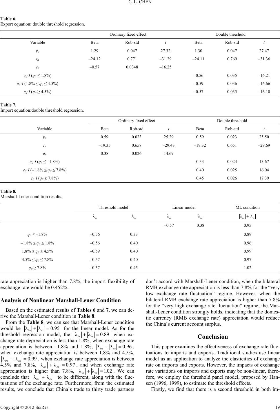. L. CHEN

Table 6.

Export equation: double threshold regression.

Ordinary fixed effect Double threshold

Variable Beta Rob-std t Beta Rob-std t

yit 1.29 0.047 27.32 1.30 0.047 27.47

tit –24.12 0.771 –31.29 –24.11 0.769 –31.36

eit –0.57 0.0348 –16.25

eit·I (qit ≤ 1.8%) –0.56 0.035 –16.21

eit·I (1.8% ≤ qit ≤ 4.5%) –0.59 0.036 –16.66

eit·I (qit ≥ 4.5%) –0.57 0.035 –16.10

Table 7.

Import equation:double threshold regression.

Ordinary fixed effect Double threshold

Variable Beta Rob-std t Beta Rob-std t

yit 0.59 0.023 25.29 0.59 0.023 25.50

tit –19.35 0.658 –29.43 –19.32 0.651 –29.69

eit 0.38 0.026 14.69

eit·I (qit ≤ –1.8%) 0.33 0.024 13.67

eit·I (–1.8% ≤ qit ≤ 7.8%) 0.40 0.025 16.04

eit·I (qit ≥ 7.8%) 0.45 0.026 17.39

Table 8.

Marshall-Lener condition results.

Threshold model Linear model ML condition

λex λim

λim λex λλ

im ex



–0.57 0.38 0.95

qit ≤ –1.8% –0.56 0.33 0.89

–1.8% ≤ qit ≤ 1.8% –0.56 0.40 0.96

1.8% ≤ qit ≤ 4.5% –0.59 0.40 0.99

4.5% ≤ qit ≤ 7.8% –0.57 0.40 0.97

qit ≥ 7.8% –0.57 0.45 1.02

rate appreciation is higher than 7.8%, the import flexibility of

exchange rate would be 0.452%.

Analysis of Nonlinear Marshall-Lener Condition

Based on the estimated results of Tables 6 and 7, we can de-

rive the Marshall-Lener condition in Table 8.

From the Table 8, we can see that Marshall-Lener condition

would be λλ0.95

im ex for the linear model. As for the

threshold regression model, the λλ0.89

im ex when ex-

change rate depreciation is less than 1.8%, when exchange rate

appreciation is between –1.8% and 1.8%, λλ0.96

im ex,

when exchange rate appreciation is between 1.8% and 4.5%,

λλ0.99

im ex, when exchange rate appreciation is between

4.5% and 7.8%, λλ0.97

im ex, and when exchange rate

appreciation is higher than 7.8%, λλ1. 0 2

im ex. We can

conclude that λλ

imex to be different, along with the fluc-

tuations of the exchange rate. Furthermore, from the estimated

results, we conclude that China’s trade to thirty trade partners

don’t accord with Marshall-Lener condition, when the bilateral

RMB exchange rate appreciation is less than 7.8% for the “very

low exchange rate fluctuation” regime. However, when the

bilateral RMB exchange rate appreciation is higher than 7.8%

for the “very high exchange rate fluctuation” regime, the Mar-

shall-Lener condition strongly holds, indicating that the domes-

tic currency (RMB exchange rate) appreciation would reduce

the China’s current account surplus.

Conclusion

This paper examines the effectiveness of exchange rate fluc-

tuations to imports and exports. Traditional studies use linear

model as an application to analyze the elasticities of exchange

rate on imports and exports. However, the impacts of exchange

rate variations on imports and exports may be non-linear, there-

fore, we employ the threshold panel model, proposed by Han-

sen (1996, 1999), to estimate the threshold effects.

Firstly, we find that there is a second threshold in both im-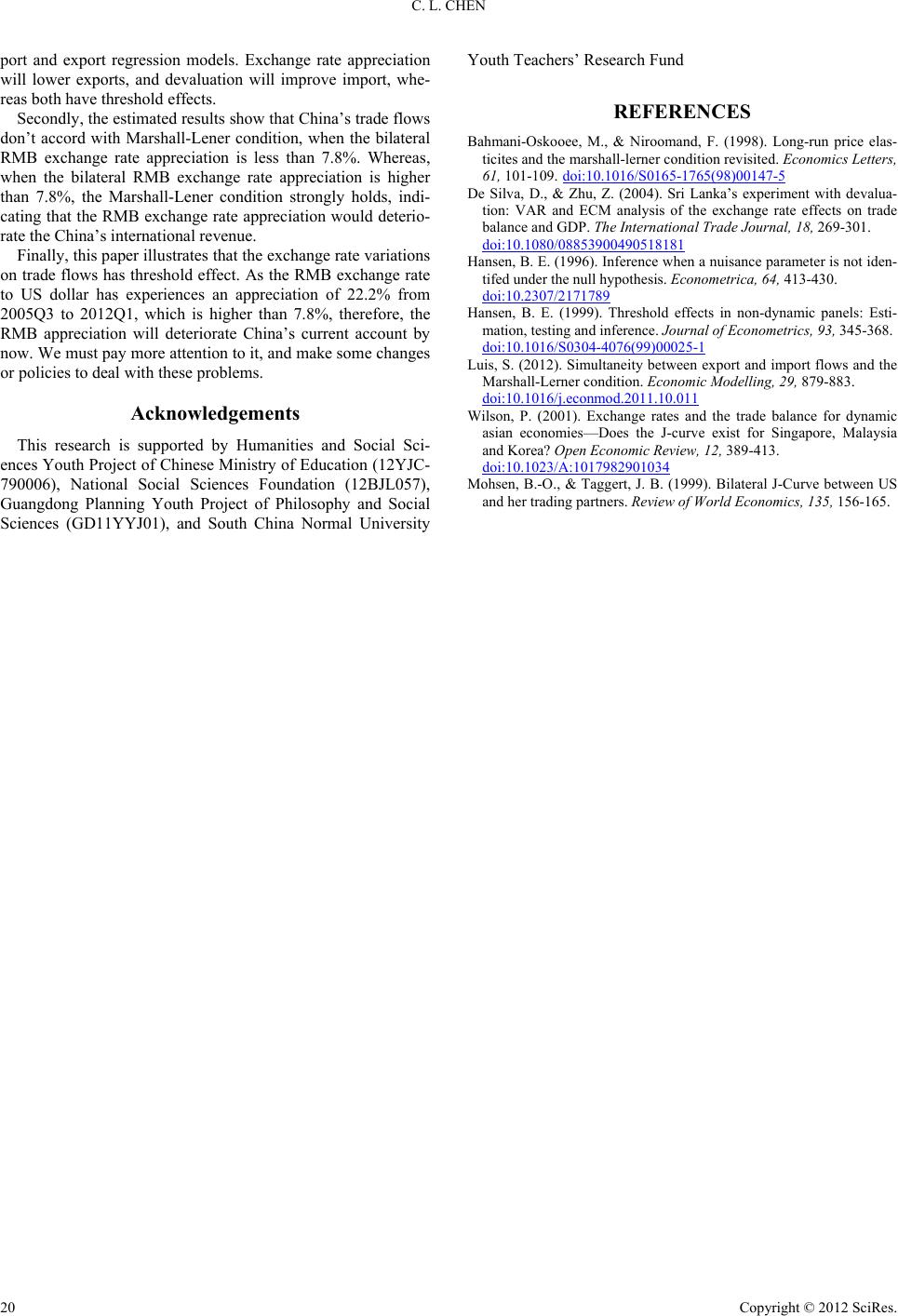

C. L. CHEN

port and export regression models. Exchange rate appreciation

will lower exports, and devaluation will improve import, whe-

reas both have threshold effects.

Secondly, the estimated results show that China’s trade flows

don’t accord with Marshall-Lener condition, when the bilateral

RMB exchange rate appreciation is less than 7.8%. Whereas,

when the bilateral RMB exchange rate appreciation is higher

than 7.8%, the Marshall-Lener condition strongly holds, indi-

cating that the RMB exchange rate appreciation would deterio-

rate the China’s international revenue.

Finally, this paper illustrates that the exchange rate variations

on trade flows has threshold effect. As the RMB exchange rate

to US dollar has experiences an appreciation of 22.2% from

2005Q3 to 2012Q1, which is higher than 7.8%, therefore, the

RMB appreciation will deteriorate China’s current account by

now. We must pay more attention to it, and make some changes

or policies to deal with these problems.

Acknowledgements

This research is supported by Humanities and Social Sci-

ences Youth Project of Chinese Ministry of Education (12YJC-

790006), National Social Sciences Foundation (12BJL057),

Guangdong Planning Youth Project of Philosophy and Social

Sciences (GD11YYJ01), and South China Normal University

Youth Teachers’ Research Fund

REFERENCES

Bahmani-Oskooee, M., & Niroomand, F. (1998). Long-run price elas-

ticites and the marshall-lerner condition revisited. Economics Letters,

61, 101-109. doi:10.1016/S0165-1765(98)00147-5

De Silva, D., & Zhu, Z. (2004). Sri Lanka’s experiment with devalua-

tion: VAR and ECM analysis of the exchange rate effects on trade

balance and GDP. The International Trade Journal, 18, 269-301.

doi:10.1080/08853900490518181

Hansen, B. E. (1996). Inference when a nuisance parameter is not iden-

tifed under the null hypothesis. Econometrica, 64, 413-430.

doi:10.2307/2171789

Hansen, B. E. (1999). Threshold effects in non-dynamic panels: Esti-

mation, testing and inference. Journal of Econometrics, 93, 345-368.

doi:10.1016/S0304-4076(99)00025-1

Luis, S. (2012). Simultaneity between export and import flows and the

Marshall-Lerner condition. Economic Modelling, 29, 879-883.

doi:10.1016/j.econmod.2011.10.011

Wilson, P. (2001). Exchange rates and the trade balance for dynamic

asian economies—Does the J-curve exist for Singapore, Malaysia

and Korea? Open Economic Review, 12, 389-413.

doi:10.1023/A:1017982901034

Mohsen, B.-O., & Taggert, J. B. (1999). Bilateral J-Curve between US

and her trading partners. Review of World Economics, 135, 156-165.