 Advances in Pure Mathematics, 2012, 2, 183-189 http://dx.doi.org/10.4236/apm.2012.23025 Published Online May 2012 (http://www.SciRP.org/journal/apm) The Best m-Term One-Sided Approximation of Besov Classes by the Trigonometric Polynomials* Rensuo Li1, Yongping Liu2# 1School of Information and Technology, Shandong Agricultural University, Tai’an, China 2School of Mathematical Sciences, Laboratory of Mathematics and Complex Systems, Ministry of Education, Beijing Normal University, Beijing, China Received December 20, 2011; revised February 5, 2012; accepted February 15, 2012 ABSTRACT In this paper, we continue studying the so called best m-term one-sided approximation and Greedy-liked one-sided ap- proximation by the trigonometric polynomials. The asymptotic estimations of the best m-terms one-sided approximation by the trigonometric polynomials on some classes of Besov spaces in the metric 1 d p LT p are given. Keywords: Besov Classes; m-Term Approximation; One-Sided Approximation; Trigonometric Polynomial; Greedy Algorithm 1. Introduction In [1,2], R. A. Devore and V. N. Temlyakov gave the asymptotic estimations of the best m-term approximation and the m-term Greedy approximation in the Besov spaces, respectively. In [3,4], by combining Ganelius’ ideas on the one-sided approximation [5] and Schmidt’s ideas on m-term approximation [6], we introduced two new concepts of the best m-term one-sided approxima- tion (Definition 2.2) and the m-term Greedy-liked one- sided approximation (Definition 2.3) and studied the problems on classes of some periodic functions defined by some multipliers. We know that the best m-term ap- proximation has many applications in adaptive PDE solvers, compression of images and signal, statistical classifica- tion, and so on, and the one-sided approximation has wide applications in conformal algorithm and operational research, etc. Hence, we are interested in the problems of the best m-term one-sided approximation and corre- sponding m-term Greedy-liked one-sided approximation. As a continuity of works in [3,4], we will study the same kinds of problems on some Besov classes in the paper. There are a lot of papers on the best m term approxi- mation problem and the best onee-sided approximation problem, we may see the papers [7-10] on the best m term approximation problem and see [11,12] on the best one-sided approximation problem. 1 :0,2π0, 2π d d TT 12 ,,, d be the d dimensional Let xx x, torus. For any two elements 12 ,,, d d yyyy R :ikx ex e, set k, ,,, d kkkkZ 11 2. 12 d, where xy denotes the inner prod- uct of x and y, i.e., 2dd yxy xyxy 1 d LT p p Denote by the space of all 2π- periodic and measurable functions f on Rd for which the following quantity 1 :d,1, p p d pT ffxxp ,, sup d xT fessfxp d p LT is a Banach space with the norm is finite. . For any , d p fLT we denote by 1 ˆd, , 2π d dk dT fkfxe x xkZ the Fourier coefficients of f (see [13]). For any positive integer m, set 1 :. d nnm m For any , d fLT 1 as Popov in [11,12], by using the multivariate Fejér kernels, 2 2 1 12 sin 2 :π2, sin 2 ,,, , d di n ii d d nx xnx xxxx T *This paper is supported by Shandong Province Higher Educational Science and Technology Program; National Natural Science Founda- tion of China (project No. 110771019); partly by the research fund for the Doctoral Program of Higher Education and partly by Beijing Natu- ral Science Foundation (Project 1102011). #Corresponding author. we defined C opyright © 2012 SciRes. APM 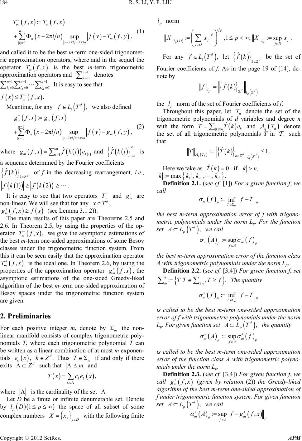 R. S. LI, Y. P. LIU 184 1 2ππ || 0 ,: , 2πsup mm n ylnn l Tfx Tfx ,, nm lnf y Tf y ,Tfx1 || 0 n l (1) and called it to be the best m-term one-sided trigonomet- ric approximation operators, where and in the sequel the operator m is the best m-term trigonometric approximation operators and denotes 12 11 00 d nn ll ,. m 1 0 . n l It is easy to see that xTfx 1, d fLT Meantime, for any we also defined 1 2ππ || 0 ,:gfx g, 2π,, sup mm n nm ylnn l fx lnfygf y 1 ˆ (2) where ,m mi ki fxf 1 ˆ i fkikie and is a sequence determined by the Fourier coefficients of f in the decreasing rearrangement, i.e., ˆ d kZ fk 12fk fk m m . It is easy to see that two operators and T are non-linear. We will see that for any , d T , m fxfx ,,Tfx ,Tfx , (see Lemma 3.1 2)). The main results of this paper are Theorems 2.5 and 2.6. In Theorem 2.5, by using the properties of the op- erator m we give the asymptotic estimations of the best m-term one-sided approximations of some Besov classes under the trigonometric function system. From this it can be seen easily that the approximation operator m is the ideal one. In Theorem 2.6, by using the properties of the approximation operator m fx x , the asymptotic estimations of the one-sided Greedy-liked algorithm of the best m-term one-sided approximation of Besov spaces under the trigonometric function system are given. 2. Preliminaries For each positive integer m, denote by m the non- linear manifold consists of complex trigonometric poly- nomials T, where each trigonometric polynomial T can be written as a linear combination of at most m exponen- tials , . Thus mk ed kZT if and only if there exits d such that m and , kk k ce x Tx where . 1p j is the cardinality of the set Let D be a finite or infinite denumerable set. Denote by the space of all subset of some p lD complex numbers D Xx with the following finite l norm 1 :,1;:. sup p p p j lDl jD jD xpXx For any 1, d fLT let ˆ d kZ fk be the set of Foficients of fthe page urier coef. As in 19 of [14], de- note by ˆ dd pp ll ffk the l norm of the set of Fourier coefficients of f. rf the tri d k Th oughout this paper, let n denote the set o gonometric polynomials of variables and degree n with the form || ˆ kn TTke and qn denote the set of all triomials n such that gonometric polyn T in ˆ :1. dd qn q kZ lZ TTk Here we take as ˆ0Tk if ,kn , . d kk k Definition 2.1. (see cf. [For a given function f, we ca 12 :max, ,k 1]) ll :inf m mp T fT the best m-term approximation error of f with trigono- metric polynomials under the norm Lp. For the function set , d p ALT we call :s up mm pp fA f the best m-term approximation error of the function class set A with trigonometric polynomials under the norm Lp. Definition 2.2. (see cf. [3,4]) For given function f, :,.TTTf The quantity 2mm :inf m mpp T fT is called to be the best m-term one-sided approximation error of f with trigonometric polynomials under the norm Lp. For given function set , d p ALT the quantity :s up mm p fA f is called to be the best m-term one-sided approximation ,4]) For given function f, we ca error of the function class A with trigonometric polyno- mials under the norm Lp. Definition 2.3. (see cf. [3 ll , m fx (given by relation (2)) the Greedy-liked algorithe best m-term one-sided approximation of f under trigonometric function system. For given function set m of th , d p ALT we call :sup p, mm fA fg fx Copyright © 2012 SciRes. APM 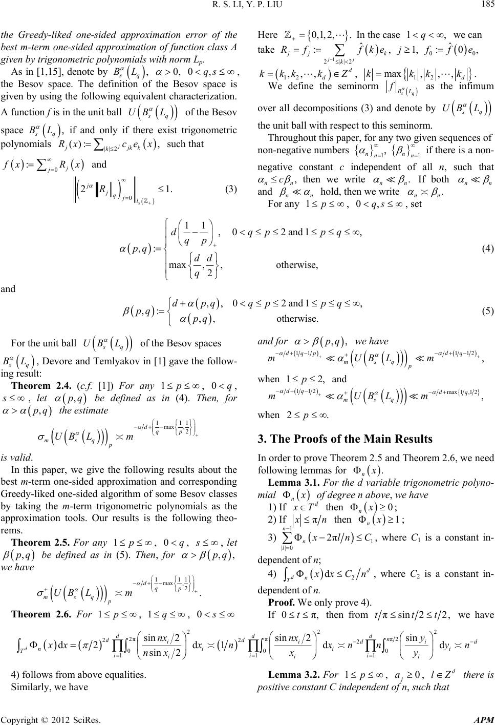 R. S. LI, Y. P. LIU Copyright © 2012 SciRes. APM 185 the Greedy-liked one-sided approximationthe best m-term one-sided approximation of function class A 0,1, 2, 1,q . In the case we can error of Here given by trigonometric polynomials with norm Lp. As in [1,15], denote by , q BL 0 , 0,qs , the Besov space. The definition of the Besov space is gi equivalent chacterizationven by using the followingar. A function f is in the unit ball sq UB L of the Besov space , q BL if and only iftrigonometric polynomials ():Rx ch that there exist ,e x suc j R x and ||2 j jjkk k 0 :j fx 0 21. s jl (3) j jq R take 1 2||2 ˆ :, jj jk k Rf fke 00 ˆ :0 fe, 1, ,,, d kkkkZ 12 d, 12 max,, ,kkkk. d We define the seminorm q L f as the infimum over all decompositions (3) and denote by sq UB L the unit ball with respect to this seminorm. Throughout this paper, for any two given sequences of 1 nn , non-negative numbers 1 nn n c if there is a non- negative constant c independent of all n, such that n , then we write n. n nn If both n and n . hold, then we write nn 1p 0,qs, For any , set 11,0 2and1, max, ,otherwise, 2 dqppq qp dd q (4) and ,:pq ,,02and1, , ,otherwise. dpq qppq pq (5) sq L of the Besov spaces ,:pq ,,pq we have For the unit ball UB q L , Devore anv in [1] gave the follow BTemlyako - ing result: d Theorem 2.4. (c.f. [1]) For any 1p, 0q , s, let ,pq be defined as in (4). Then, for ,pq the estimate 111 max ,d q UB L 2qp ms p m is valid. In this paper, we give the following results about the one-sided approximation and corresponding G best m-term reedy-liked one-sided algorithm of some Besov classes by taking the m-term trigonometric polynomials as the approximation tools. Our results is the following theo- rems. Theorem 2.5. For any 1p, 0q, s , let ,pq be defined as in (5). Then, for ,,pq w e have 11 maxd 1 ,2. qp ms UBL q p m 2.6. For , 0s and for 11 112 , dqpdq ms p m q mUBL when 12,p and 1p , Theorem 1q 112 max1,12, dq dq sq BLm when 2.p m mU e Proofsf the Main Results 2.6, we need 3. Th o In order to prove Theorem 2.5 and Theorem following lemmas for . n Lemma 3.1. For the d variable trigonometric polyno- mial n of degreee n abov, we have 1) If d T then 0 nx ; 2) If π n then 1 nx ; 3) 1 0 n 1n || 2π l ln C , wheC1 is a constant in- dedent of n; re pen 4) 2 d d dn T xC de dent of n. n , where C2 is a constant in- of. We only prove 4). pen Pro If 0π,t then from πsin 22,ttt we have 2 2 sin d2 d 22 πππ2 2 22 000 111 2in 2sin 1 d sin 2 d ddn dd iii niii Tiii iii nx nxysd d dd x xn ny nxx y xnn 4) follows from above equalities. Similarly, we have Lemma 3.2. For 1p , 0 j a, d lZ there is positive constant C independent of n, such that 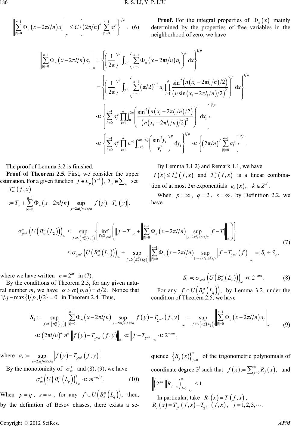 R. S. LI, Y. P. LIU 186 1 11 || 0 π. || 0 2π2 nn dp l l n a (6) Proof. For the integral properties of n nl p xlnaC l mainly determined by the properties of free variables in the neighborhood of zero, we have 1 2πd p p l 1 1d n 1 || 0|| 0 1 2 12 2 || 01 2 12π 0 || 01 2π 2π 2π2 sin 1π2d 2πsin 2π2 2π2 sin 2 d d n nl n T ll p p dd ndii l Tliii d nii p l lii xlna nxl n ax nx ln nxl n a nx xlnax 1 2 11 2 11 ππ 1 2 π || 0|| 0 1 d π2 sin d2π. i i p p i i p pp d nn nl d pp i lil l ll ii x ln y anyn a y The proof of Lemma 3.2 is finished. Proof of Theorem 2.5. First, we consider the upper estimation. For a given function d p LT, mm T set 1n |2π|π || 0 :2π. sup mn m ylnn l Tx ln fyTy , m Tfx By Lemma 3.1 2) and Remark 1.1, we have , m xTfx and , m Tfx is a linear combina- tion of at most 2m exponentials , k ex d kZ. When p , 2q , , by Definition ve 2.2, we ha 2 2 1 |2π|π || 0 1 212 2 2 |2π|π || 0 inf up 2π:, sup sup md md md n Tylnn l n n ylnn l fUB L f TlnT Lxlnf TfSS (7) ere we hm (7). y the for any given natu- have 2 2 2sup md fU B L UBL UB 2πs nx f wh B ave written conditions 2 in eorem 2.5, n of Th ral number m, we ,2.pqd Notice that 1max1,120qp in Theorem 2.4. Thus, 12 2 :2. md m SUBL For any (8) , sq fUBL by Lemma 3.2, under the condition of Theorem 2.5, we have 1 2 |2π|π :2π sup sup q n ylnn fUB L ddm Sx lnf 1 ||=0 ||= 2 2 sup 2π,2, md n n l l fU B L md y T lnnfyTfyfT 20 ,2π md q nl f yxlna (9) where 2 |2π|π :,. sup md l ylnn afyTfy By the monotonicity of m and (8), (9), we have . d msq UB Lm (10) y ,fUBL then, e- quence 0 j When pq, , for ansq the definition of Besov classes, there exists a sby Rx of the trigonometric polyno coordinate degree 2j such that 0 :, j j mials of xRx and 1 21. j jpjl R In particular, take 01 ,Rx Tfx, 1 22 ,, jj j RxTfx Tfx , 1, 2,3,.j Copyright © 2012 SciRes. APM  R. S. LI, Y. P. LIU 187 Here er , mfx ar trigo- nometric approximation operators in (1). From the rela- the opator Te the best m-term tioapproximation and non-linear ap- proximation and Lemma 3.2, whave n between linear e 2 2md md 2md p pp 1 |2π|π || =0 1 1 =1 ||=0 1 =1 ||=0 inf sup 2π sup sup 22 2π sup sup 22π q q qq ppg fUB L n nj ylnn ljm fUB Lp n jj jnl p jm l fUB LfUB L n d j jm l UB Lfg lnR y Rlna na EUB L 1 12 :. p p lSS (11) Here |2π|π1. sup lj ylnn jm aRy Under the condition of Theorem 2.5, it is easy to see that 22. jm 1 1 jm S (12) . Set hy Next, 1, j jm R y and we will estimate 2 S 1 1 ,2π ,1d . sup d p pTyUx n hnhyhxx Since the measure of the neighborhood 1 2π2π ππ 2π,π, dii i jj Ujnn nnnn is 2πd n, so, by the definition of Besov classes and Minkowskii inequality, we have 11 1 22π,ππ,π2π,π || 0|| 0 1 2π,π2π,π || 0 1 1 2π,π2π,π|| 0 :d d sup sup d sup pp n U lnnlnn yUln n ll p n Ulnn yUln n l p p n n UlnnyUlnnl Sfahyx hy x hy hxx 1 2 : n p lU x 1 h || 0l d p hx x p 1 1 2π,π 1 1 1 ,2π d dd,1. sup dd p Ulnn p pp p pp TT yUx n hx x hyhxxhxxh nh For a fixed 12 ,, , d d set 12 || 12 . d d D xx By the mathematical induction d, it is easy to see that on || ||1 . d ss1,1 p Rn Notice that 2m n n DR . From modulus [12] and Bernstein i the properties of smooth nequality, we have |||| || 11 11||1 1||1 1||1 ,1 2 . dd s ss p || || ,1 222 s 1 2 2 p sm smsm p jd sp sm hnnn DRnR R By the conditions of Theorem 2.5, and α > d, we have dsss R n m j 1,12 m p hn From (11), (12) and (3), we have 2. m p h Copyright © 2012 SciRes. APM 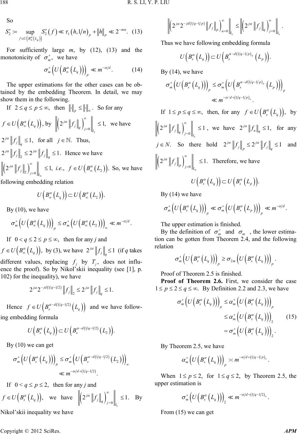 R. S. LI, Y. P. LIU 188 So 221 :, sup q p fU B L SSfh 12. m p nh (13) For sufficiently large m, by (12), (13) and the mcity of , m onotoni we have . d UB Lm (14) mqp r cases can be ob- tai In detail, we may show them in the following. ,en The upper estimations for the othe ned by the embedding Theore.m If 2qp th. p So for any B q L, by fU 0 21, j jqjl f we have s 21, j jq f for all .j Thus, 2 221. jj jj q ff Hence we have 20 21, j jjl f i.e., 2. UB L So, we have following embedding relation 2. q L L ave UB UB By (10), we h 2 p LUBL then for any j and (3), we hav . d m 02 ,qp , q L by mq m UB If fUB e21 j jq f different valu, repl (if q takes es acing by , T does not influ- ii inequality (see [1], p. 102) for the inequality), we have ence the proof). So by Nikol’sk 112 2 22 jd q 2 1. jj jj q ff Hence 112dq sq L and we have folw- ing embedding formula fUB lo 112dq q sL 2. s UB LUB By (10) we can get 11 2 . dq m 112 2 dq msq ms p UB LUBL 0< 2,qp then for any j and L If sq UB , we have f =0 21 s jqjl . jf By Nikol’skii inequality we have 11 00 222 . s jd qp jj jj pq nj ll ff Thus we have following embedding formula 11 . dq p sq sp UB LUBL By (14), we have 11 /11 . dqp ms pmsq p dqp UB L m If 1,pq UBL , sq fUBL by then, for any =0 s jqjl f 21 j , we have 2 j n f 1, q for any .jN 221 j jj pq ff and j So there hold 0 21. j jpjl f Therefore, we have . sqsp UB LUB L By (14) we have . d mspmsq pp UB LUB Lm The upper estimation is finished. By the definition of m and m , the lower estima- tion can be gotten from Theorem 2.4, and the following relation 2. msqmsq p UBB L Proof of Theorem. Proof of Theorem 2.6. First, we consider the case 1p L U 2.5 is finished 2 .qition 2.2 and 2.3, we ha By Definve q msq 2 2 . ms p ms msq UBL UBL UBL (15) By Theorem 2.5, we have q UB L 11 . dqp UB Lm ms q p When 12,p for 2q1 , by Theorem 2.5, the upper estimation is 112 2 . dq msq UB Lm From (15) we can get Copyright © 2012 SciRes. APM  R. S. LI, Y. P. LIU Copyright © 2012 SciRes. APM 189 112dq 2 . ms q msq p mUB LUBL ) , 12q, by the relation between -tximation and Greedy algorithm [7], we have (16 Whe best m n 2p erm appro 1. p mm 12 p gf mf (17) For , sq fUBL and any l, by (16), (17) and Theorem 2.4, we have |2π|π 121 12 sup lm ylnn dq gfy (18) :, . m afy fgmmm From Lemma 3.2 and relation (17), (18), w e have 1 2πsup n n |2π|π || 0 1 112/1 121 sup . sq ms q mm p pylnn l fUB L dqp dq dq f gf g mm mmmm r the case 2.q xy ln UBL When 2,p we conside By the 2, jj q ff we have 2. ssq UB LUB L (20) By (19) and (20), we can get 12 2. d msqms p p UB LUB Lm (21) In the following we will give the lower estimation. By on 2.3, we have . Definiti 2msqmsq p UBL UBL And by Theorem 2.4, we have 11dqp when 12,p and ms q p UB Lm 112dq msq p UB Lm w 2.6. REFERENCES lyakov, “Nonlinear ums,” Journal of Fourier Analysis Application, Vol. 2, No. 1, 1995, pp. 29-48. hen 2.p This finishes the proof of Theorem [1] proximation by Trigonometric S R. A. Devore and V. N. Tem Ap- doi:10.1007/s00041-001-4021-8 . N. Temlyakov, “Greedy Algorithm and m-Term Trigo- nometric Approximation,” Constructive Approximation Vol. 14, No. 4, 1998, pp. 569-587. oi:10.1007/s003659900090 [2] V , d [3] Estimations of of Function Classes DetermineAdvance in Mathematics (008, pp. 211-221. Series, Vol. 26, No. 5, 2010, pp. 975-984. doi:10.1007/s10114-009-6478-3 [5] T. Ganelius, “On One-Sided Approximation by Trigono- metrical Polynomials,” Mathematica Scandinavica, Vol. 4, 1956, pp. 247-258. [6] E. Schmidt, “Zur Theorie der Linearen und Nichtlinearen Integralgleichungen,” Annals of Mathematics, Vol. 63, 1907, pp. 433-476. doi:10.1007/BF01449770 [7] A. S. Romanyuk, “Best m-Term Trigonometric Approxi- mations of Besov Classes of Periodic Functions of Sev- eral Variables,” Izvestiya: Mathematics, Vol. 67, No. 2, 2003, pp. 265-302. doi:10.1070/IM2003v067n02ABEH000427 [8] S. V. Konyagin and V. N. Temlyakov, “Convergence of Greedy Approximation II. The Trigonometric Systerm,” Studia Mathematica, Vol. 159, No. 2, 2003, pp. 161-184. doi:10.4064/sm159-2-1 [9] V. N. Temlyakov, “The Best m-Term Approximation and Greedy Algorithms,” Advances in Computational Math- ematics, Vol. 8, No. 3, 1998, pp. 249-265. doi:10.1023/A:1018900431309 [10] R. Li and Y. Liu, “The Asymptotic Estimations of Best .089 m-Term Approximation and Greedy Algorithm for Mul- tiplier Function Classes Defined by Fourier Series,” Chi- nese Journal of Engineering Mathematics, Vol. 25, No. 1, 2008, pp. 89-96. doi:10.3901/JME.2008.10 R. S. Li and Y. P. Liu, “The Asymptotic Best m-Term One-Sided Approximation d by Fourier Coefficients,” China), Vol. 37, No. 2, 2 [4] R. Li and Y. Liu, “Best m-Term One-Sided Trigonomet- ric Approximation of Some Function Classes Defined by a Kind of Multipliers,” Acta Mathematica Sinica, English mation of Periodic Func- One-Sided Approximation of Mul- , Heidelberg, [11] V. A. Popov, “Onesided Approxi tions of Serveral Variables,” Comptes Rendus de Academie Bulgare Sciences, Vol. 35, No. 12, 1982, pp. 1639-1642. [12] V. A. Popov, “On the tivariate Functions,” In: C. K. Chui, L. L. Schumaker and J. D. Ward, Eds., Approximation Theory IV, Academic Press, New York, 1983. [13] A. Zygmund, “Trigonometric Series II,” Cambridge Uni- versity Press, New York, 1959. [14] R. A. Devore and G. G. Lorentz, “Constructive Approxi- mation,” Spring-Verlag, New York, Berlin 1993. [15] R. A. Devore and V. Popov, “Interpolation of Besov Spaces,” American Mathematical Society, Vol. 305, No. 1, 1988, pp. 397-414.
|

