Generation Reliability Evaluation in Deregulated Power Systems Using Game Theory and Neural Networks

doi:10.4236/sgre.2012.32013

Paper Menu >>

Journal Menu >>

Smart Grid and Renewable Energy, 2012, 3, 89-95

http://dx.doi.org/10.4236/sgre.2012.32013 Published Online May 2012 (http://www.SciRP.org/journal/sgre) 1

Generation Reliability Evaluation in Deregulated Power

Systems Using Game Theory and Neural Networks

Hossein Haroonabadi1, Hassan Barati2

1Electrical Department, Islamic Azad University (Islamshahr Branch), Tehran, Iran; 2Electric al Department, Isla mic Azad University

(Dezful Branch), Dezful, Iran.

Email: [email protected]c.ir, [email protected]

Received March 30th, 2012; revised April 27th, 2012; accepted May 4th, 2012

ABSTRACT

Deregulation policy has caused some changes in the concepts of power systems reliability assessment and enhancement.

In the present research, generation reliability is considered, and a method for its assessment is proposed using Game

Theory (GT) and Neural Networks (NN). Also, due to the stochastic behavior of power markets and generators’ forced

outages, Monte Carlo Simulation (MCS) is used for reliability evaluation. Generation reliability focuses merely on the

interaction between generation complex and load. Therefore, in the research, based on the behavior of players in the

market and using GT, two outco mes are con sider ed : co op eration and non-co op eratio n. Th e proposed meth od is assessed

on IEEE-Reliability Test System with satisfactory results. Loss of Load Expectation (LOLE) is used as the reliability

index and the resu lts show generation reliability in cooperation market is better than non-coop eration outcome.

Keywords: Power Market; Generation Reliability; Game Theory (GT); Neural Networks (NN); Monte Carlo

Simulation (MCS)

1. Introduction

Power systems have evolved over decades. Their primary

emphasis is on providing a reliable and economic supply

of electrical energy to their customers [1]. A real power

system is complex, highly integrated and almost very

large. It is divided into appropriate subsystems or func-

tional zones that can be analyzed separately [1]. This

paper deals with generation reliability assessment (Hier-

archical Level I-HLI) in power pool market, and the trans-

mission and distribution systems are considered reliable

and adequate as shown in Figure 1.

Most of the methods used for generation reliability

evaluation are based on the loss of load or energy ap-

proach. One of the suitable indices that describes genera-

tion reliability level is “Loss of Load Expectation” (LOLE),

that is the time in which load is more than the available

generation capacity.

Reliabl e Transmis-

si on & Di stribution

Systems

Ge n. 1

Ge n. 2

Ge n. n

Load

Figure 1. Power pool market schematic for HLI reliability

assessment.

Generally, the reliability indices of a system can be

evaluated using one of the following two basic approaches

[1]:

 Analytical techniques,

 Stochastic simulation.

Simulation techniques estimate the reliability indices

by simulating the actual process and random behavior of

the system. Since power markets and generators’ forced

outages have stochastic behavior, Monte Carlo Simula-

tion (MCS), as one of the most powerful methods for

statistical analysis of stochastic problems, is used for

reliability assessment in this research.

Since the beginning of the 21st century, many countries

have been trying to deregulate their power systems and

create power markets [2,3]. In the power markets, the

main function of players is their own profit maximization,

which severely depends on the type of the market. As a

result, generation reliability assessment depends on the

market’s type and characteristics.

Reliability problems have been evaluated in power

markets during the last decade [4,5]. This paper deals

with generation reliability in power pool markets using

game theory (GT) and Neural Networks (NN). GT is the

mathematical study of interaction among independent,

self-interested agents [6]. That is, where the actions of

one agent affect the payoff (utility or profit) of another

agent in a way that affects the choice of best action by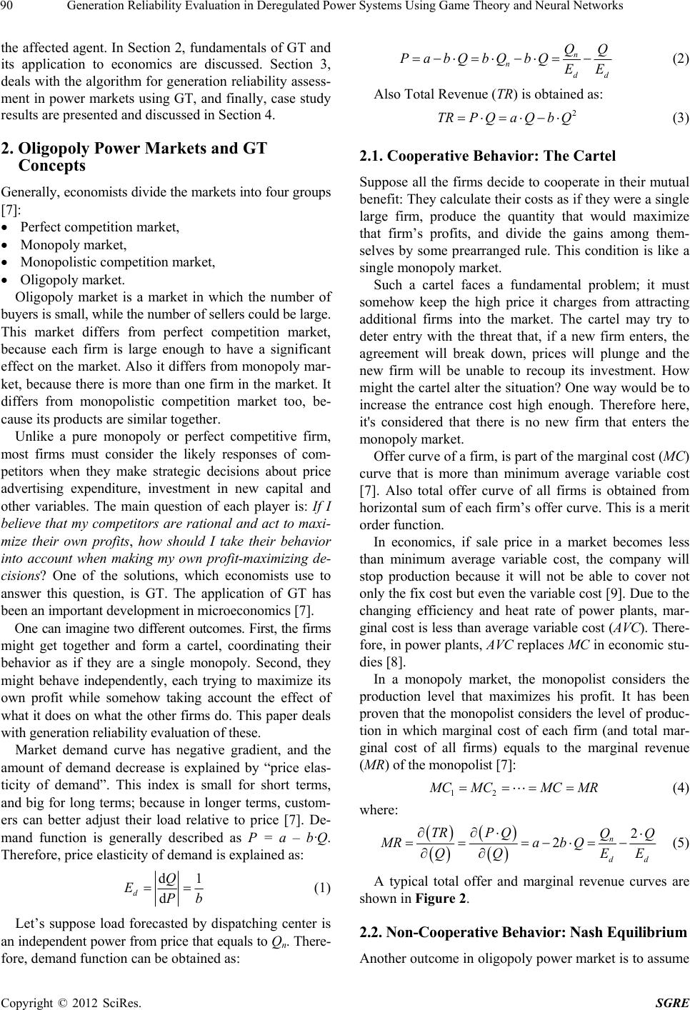

Generation Reliability Evaluation in Deregulated Power Systems Using Game Theory and Neural Networks

the affected agent. In Section 2, fundamentals of GT and

its application to economics are discussed. Section 3,

deals with the algorithm for generation reliability assess-

ment in power markets using GT, and finally, case study

results are presented and discussed in Section 4.

2. Oligopoly Power Markets and GT

Concepts

Generally, economists divide the markets into four groups

[7]:

 Perfect competition market,

 Monopoly market,

 Monopolistic competition market,

 Oligopoly market.

Oligopoly market is a market in which the number of

buyers is small, while the number of sellers could be large.

This market differs from perfect competition market,

because each firm is large enough to have a significant

effect on the market. Also it differs from monopoly mar-

ket, because there is more than one firm in the market. It

differs from monopolistic competition market too, be-

cause its products are similar together.

Unlike a pure monopoly or perfect competitive firm,

most firms must consider the likely responses of com-

petitors when they make strategic decisions about price

advertising expenditure, investment in new capital and

other variables. The main question of each player is: If I

believe that my competitors are rational and act to maxi-

mize their own profits, how should I take their behavior

into account when making my own profit-maximizing de-

cisions? One of the solutions, which economists use to

answer this question, is GT. The application of GT has

been an important devel opment in mi croeconomics [7].

One can imag ine two different outcomes . First, the firms

might get together and form a cartel, coordinating their

behavior as if they are a single monopoly. Second, they

might behave independently, each trying to maximize its

own profit while somehow taking account the effect of

what it does on what the other firms do. This paper deals

with generation reliability evaluation of these.

Market demand curve has negative gradient, and the

amount of demand decrease is explained by “price elas-

ticity of demand”. This index is small for short terms,

and big for long terms; because in longer terms, custom-

ers can better adjust their load relative to price [7]. De-

mand function is generally described as P = a – b·Q.

Therefore, price elasticity of demand is explained as:

EPb



(1)

Let’s suppose load forecasted by dispatching center is

an independent power from price that equals to Qn. There-

fore, dem a nd function can be obt ai n ed as:

ndd

Pa bQbQbQEE

   (2)

Also Total Revenue (TR) is obtained as:

TRP Qa Qb Q



 (3)

2.1. Cooperative Behavior: The Cartel

Suppose all the firms decide to cooperate in their mutual

benefit: They calculate their co sts as if they were a single

large firm, produce the quantity that would maximize

that firm’s profits, and divide the gains among them-

selves by some prearranged rule. This condition is like a

single monopoly market.

Such a cartel faces a fundamental problem; it must

somehow keep the high price it charges from attracting

additional firms into the market. The cartel may try to

deter entry with the threat that, if a new firm enters, the

agreement will break down, prices will plunge and the

new firm will be unable to recoup its investment. How

might the cartel alter the situatio n? One way would be to

increase the entrance cost high enough. Therefore here,

it's considered that there is no new firm that enters the

monopoly market.

Offer curve of a firm, is part of the marginal cost (MC)

curve that is more than minimum average variable cost

[7]. Also total offer curve of all firms is obtained from

horizontal sum of each firm’s offer curve. This is a merit

order function.

In economics, if sale price in a market becomes less

than minimum average variable cost, the company will

stop production because it will not be able to cover not

only the fix cost but even the variable cost [9]. Due to the

changing efficiency and heat rate of power plants, mar-

ginal cost is le ss than average variable cost (AVC). There-

fore, in power plants, AVC replaces MC in economic stu-

dies [8].

In a monopoly market, the monopolist considers the

production level that maximizes his profit. It has been

proven that the monopolist considers the level of produc-

tion in which marginal cost of each firm (and total mar-

ginal cost of all firms) equals to the marginal revenue

(MR) of the monopolist [7]:

CMC MCMR



  (4)

where:













TRP QQQ

MRab Q

QQ E





 

 (5)

A typical total offer and marginal revenue curves are

shown in Figure 2.

2.2. Non-Cooperative Behavior: Nash Equilibrium

Another outcome in oligopoly power market is to assume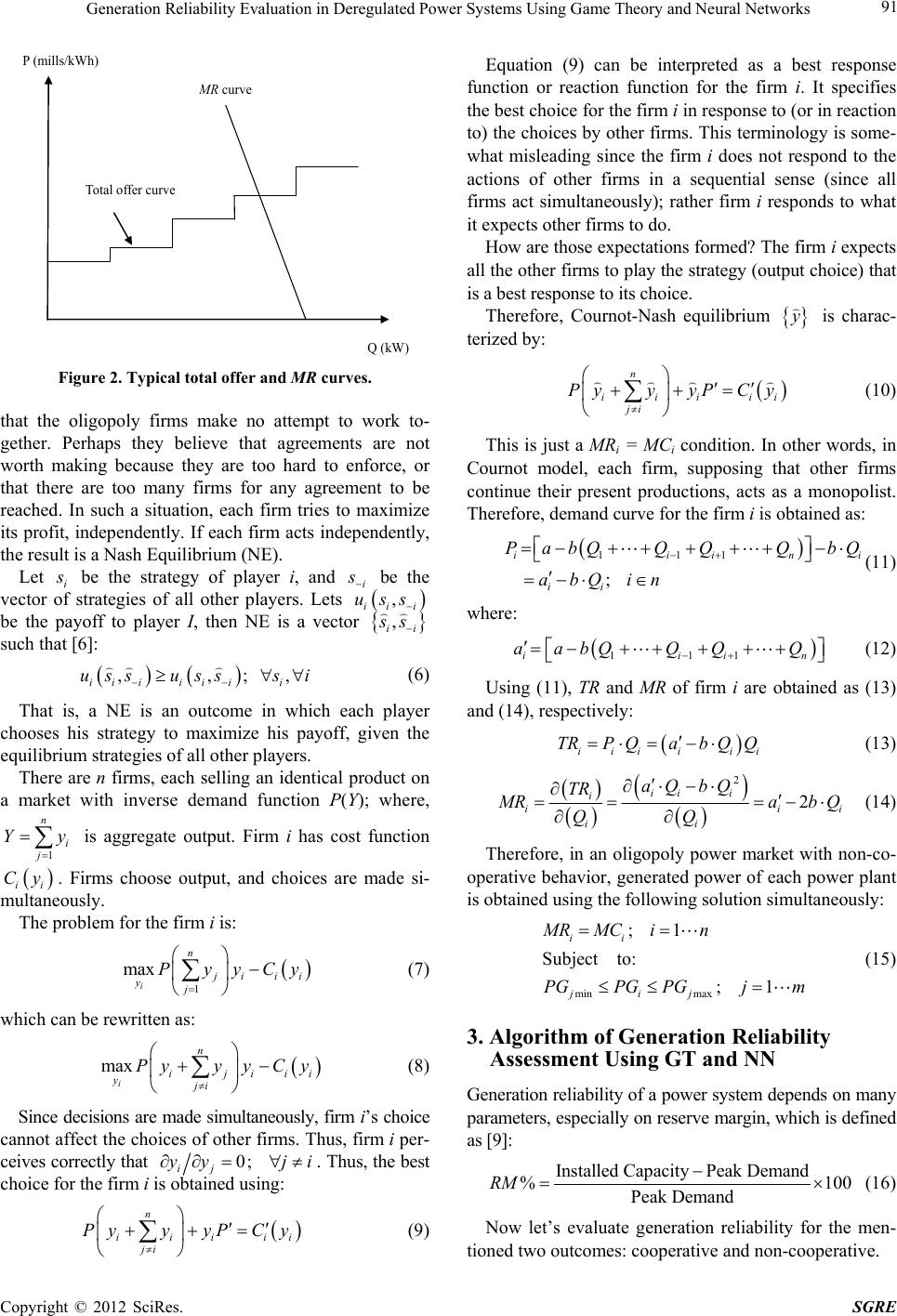

Generation Reliability Evaluation in Deregulated Power Systems Using Game Theory and Neural Networks 91

MR curve

Total offer curve

P (mills/kWh)

Q (kW)

Figure 2. Typical total offer and MR curves.

that the oligopoly firms make no attempt to work to-

gether. Perhaps they believe that agreements are not

worth making because they are too hard to enforce, or

that there are too many firms for any agreement to be

reached. In such a situation, each firm tries to maximize

its profit, independently. If each firm acts independently,

the result is a Nash Equilibrium (NE).

Let i

be the strategy of player i, and i



be the

vector of strategies of all other players. Lets





ii i

uss



be the payoff to player I, then NE is a vector





s



such that [6]:



,,;

ii iii ii

ussusss i



,



 (6)

That is, a NE is an outcome in which each player

chooses his strategy to maximize his payoff, given the

equilibrium strategies of all other players.

There are n firms, each selling an identical product on

a market with inverse demand function P(Y); where,



y is aggregate output. Firm i has cost function



Cy. Firms choose output, and choices are made si-

multaneously.

The problem for the firm i is:



max

iii

PyyCy











 (7)

which can be rewritten as:



max

ijii

yji

Pyy yCy











i

(8)

Since decisions are made simultaneously, firm i’s choice

cannot affect the choices of other firms. Thus, firm i per-

ceives correctly that 0;

yy ji . Thus, the best

choice for the firm i is obtained using:



iiii

PyyyP Cy















Equation (9) can be interpreted as a best response

function or reaction function for the firm i. It specifies

the best choice for the firm i in response to (or in reaction

to) the choices by other firms. This terminology is some-

what misleading since the firm i does not respond to the

actions of other firms in a sequential sense (since all

firms act simultaneously); rather firm i responds to what

it expects other firms to do.

How are those expectations formed? The firm i expects

all the other firms to play the strategy (output choice) that

is a best response to its choice.

Therefore, Cournot-Nash equilibrium





is charac-

terized by:



iiii

PyyyP Cy













i



 

(10)

This is just a MRi = MCi condition. In other words, in

Cournot model, each firm, supposing that other firms

continue their present productions, acts as a monopolist.

Therefore, demand curve for the firm i is obtained as:





111

;

iiin

PabQQ QQbQ

abQin













 

 (11)

where:





111iii

aabQ QQQ



n













(12)

Using (11), TR and MR of firm i are obtained as (13)

and (14), respectively:





iii ii

TRPQab QQ



 i

(13)









ii i

aQ bQ





bQ





  (14)

Therefore, in an oligopoly power market with non-co-

operative behavior, generated power of each power plant

is obtained using the follo wing solution simultaneously:

min max

Subject to:

jij

MR MCin

PGPG PGjm



 



(15)

3. Algorithm of Generation Reliability

Assessment Using GT and NN

Generation reliability of a power system depends on many

parameters, especially on reserve margin, which is defined

as [9]:

Installed CapacityPeak Demand

Peak Demand

RM 

00

(16)

Now let’s evaluate generation reliability for the men-

tioned two outcomes: cooperative and non-cooperative.

(9)

Generation Reliability Evaluation in Deregulated Power Systems Using Game Theory and Neural Networks

3.1. Generation Reliability Assessment in

Cooperative Condition (Monopoly Market)

As explained before, in cooperative outcome, the market

acts as a monopoly market. The algorithm of generation

reliability assessment in monopoly power pool market

using Monte Carlo simulation is as follows:

1) Calculate total offer curve of the power plants.

2) Select a random day and its load (Qn), and calculate

MR curve using (5).

3) The power plants, selected for generation in the se-

lected day, are determined from the intersection of the

power plants’ total offer curve and MR cu rve with regard

to the reserve margin.

4) For each power plant selected in the previous step, a

random number between 0 - 1 is generated. If the gener-

ated number is more than the power plant’s Forced Out-

age Rate (FOR), the power plant is considered as avail-

able in the mentioned iteration; otherwise, it encounters

forced outage and thus can not generate power. This

process is performed for all power plants using an inde-

pendent random number generated for each plant. Finally,

sum of the available power plants’ generation capacities

is calculated. If the sum becomes less than the intersec-

tion of the power plants’ total offer curve and demand

exponent curve, we will have interrup tion in th e iteration,

and therefore, LOLE will increase by as much as one unit;

otherwise, we will go to the next iteration. The algorithm

of available generated power and LOLE calculation for

each iteration in MCS is shown in Figure 3.

5) The Steps 2 to 4 are repeated for calculation of the

final LOLE.

3.2. Generation Reliability Assessment in

Non-Cooperative Condition (Cournot-Nash

Equilibrium)

The algorithm of generation reliability assessment in oli-

gopoly power pool market for non-cooperation outcome

using MCS is as follows:

1) Select a random day and its load (Qn), and calculate

demand curve cross of basis and gradient using (2).

2) Calculate the power plants’ generated powers in the

selected day using (11)-(15). Also, the amount of total

demand is obtained using sum of plants’ generated pow-

ers regard l es s of rese r v e margi n .

3) For each power plant selected in the previous step,

with regard to the reserve margin, a random number be-

tween 0 - 1 is generated. If the generated number is more

than the power plant’s Forced Outage Rate (FOR), the

power plant is considered as available in the mentioned

iteration; otherwise, it encounters forced outage and thus

can not generate power. This process is performed for all

power plants using an independent random number gen-

erated for each plant. Finally, sum of the available power

Generate a random number

between [0-1] (U

)

Select the first generator (i = 1);

Available Generated Power (AGP) = 0;

LOLE = 0

AG P = AGP + P G

>= FOR

i = NG

i = i + 1

Total AGP calculation

AGP < Load

LOLE = LOLE + 1 LOLE does not change

Figure 3. The algorithm of available generated power and

LOLE calculation for each iteration using MCS.

plants’ generation capacities is calculated. If the sum

becomes less than the intersection of the power plants’

total offer curve and demand exponent curve, we will

have interruption in the iteration, and therefore, LOLE

will increase by as much as one unit; otherwise, we will

go to the next iteration.

4) Steps 1-3 are repeated for calculation of the final

LOLE.

3.3. Generation Reliability Evaluation Using NN

Now, to create a unique structure, a four-layer Perceptron

NN is used for reliability evaluation. Th e number of neu-

rons in each layer is 20, 15, 10 and 1, respectively (Fig-

ure 4). All neurons in the first, third and last layers have

POSLIN transfer function, and the second layer has

TANSIG transfer function. Three inputs of the NN in-

clude:

 C: A number that shows the kind of outcome (1 for

cooperative, and 2 for non-cooperative outcomes),

 Ed: Price elasticity of demand,

 RM: Reserve margin.

Also, the NN’s output is LOLE index.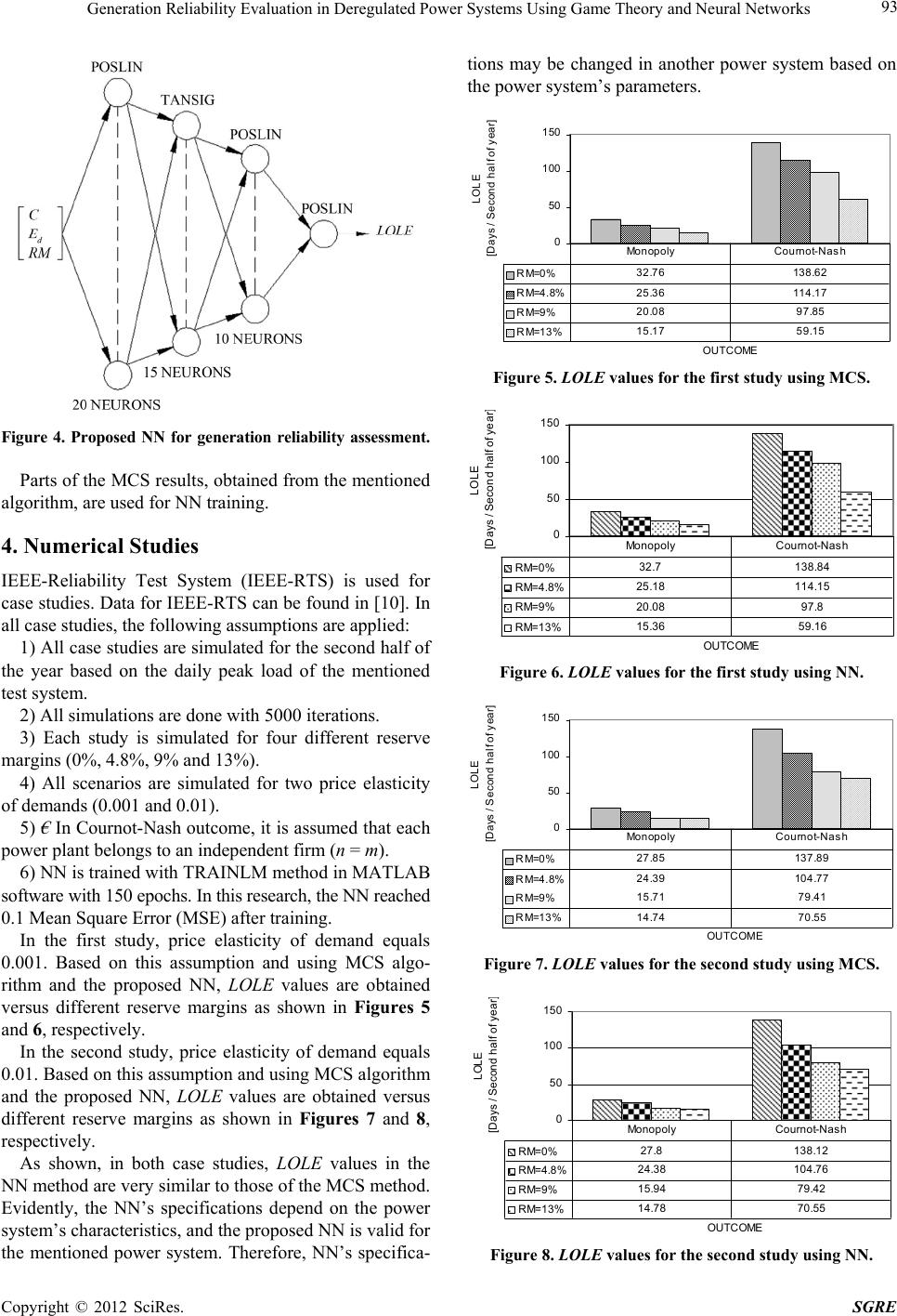

Generation Reliability Evaluation in Deregulated Power Systems Using Game Theory and Neural Networks 93

Figure 4. Proposed NN for generation reliability assessment.

Parts of the MCS results, obtained from the mentioned

algorithm, are used for NN training.

4. Numerical Studies

IEEE-Reliability Test System (IEEE-RTS) is used for

case studies. Data for IEEE-RTS can be found in [10]. In

all case studies, the following assumptions are applied:

1) All case studies are simulated for the second half of

the year based on the daily peak load of the mentioned

test system.

2) All simulations are done with 5000 iterations.

3) Each study is simulated for four different reserve

margins (0%, 4.8%, 9% and 13%).

4) All scenarios are simulated for two price elasticity

of demands (0.001 and 0.01).

5) € In Cournot-Nash outcome, it is assumed that each

power plant belongs to an independent firm (n = m).

6) NN is trained with TRAINLM method in MATLAB

software with 150 epochs. In this research, the NN reached

0.1 Mean Square Error (MSE) after training.

In the first study, price elasticity of demand equals

0.001. Based on this assumption and using MCS algo-

rithm and the proposed NN, LOLE values are obtained

versus different reserve margins as shown in Figures 5

and 6, respectively.

In the second study, price elasticity of demand equals

0.01. Based on this assumption and using MCS algorithm

and the proposed NN, LOLE values are obtained versus

different reserve margins as shown in Figures 7 and 8,

respectively.

As shown, in both case studies, LOLE values in the

NN method are very similar to those of the MCS method.

Evidently, the NN’s specifications depend on the power

system’s characteristics, and the proposed NN is valid for

the mentioned power system. Therefore, NN’s specifica-

tions may be changed in another power system based on

the power system’s parameters.

100

150

OUTCOM E

LOLE

[Days / S econd half of ye ar]

RM=0% 32.76 138.62

RM=4.8%25.36114.17

RM=9% 20.08 97.85

RM=13% 15.1759.15

Monopoly Cournot-Nash

Figure 5. LOLE values for the first study using MCS.

100

150

OUTCOME

LOLE

[ Day s / Sec ond half of year

]

RM=0% 32.7 138.84

RM=4.8% 25.18 114.15

RM=9% 20.08 97.8

RM=13% 15.36 59.16

Monopoly Cournot-Nash

Figure 6. LOLE values for the first study using NN.

100

150

OUTCOME

LOLE

[Days / Sec o nd half of y ear ]

RM=0% 27.85 137.89

RM=4.8% 24.39 104.77

RM=9% 15.71 79.41

RM=13% 14.74 70.55

Monopoly Cournot-Nash

Figure 7. LOLE values for the second study using M CS.

100

150

OUTCOME

LOLE

[Days / Second half of year

]

RM=0%27.8 138.12

RM=4.8% 24.38 104.76

RM=9% 15.94 79.42

RM=13%14.78 70.55

Monopoly Cournot-Nash

Figure 8. LOLE values for the second study using NN.

Generation Reliability Evaluation in Deregulated Power Systems Using Game Theory and Neural Networks

In both case studies, if reserve margin increases, LOLE

will decrease and reliability will improve.

In monopoly market, if price elasticity increases, MR

curve takes less gradient. As a result, intersection of the

power plants’ total offer curve and MR curve occurs at

less demand. This leads to the operation of fewer power

plants. Therefore, in all case studies in monopoly market,

if price elasticity increases, LOLE will decrease.

In Cournot-Nash equilibrium, if price elasticity varies,

the generated power of every power plant varies, too.

Therefore, LOLE will differ based on the share of every

plant’s generated power and FOR.

LOLE values in Cournot-Nash outcome are very big-

ger than those of the monopoly outcome. Because in mo-

nopoly market, only the plants, which are selected by in-

tersection of the total offer and MR curves, are in service

(considering RM), while in Cournot-Nash outcome, all of

the players participate in the market, and the load feeds

based on the plants’ optimum generated power. Therefore,

in monopoly market, at every time period, only a few

plants are in service, while in Cournot-Nash ou tcome, all

of the power plants are in service based on their optimum

generation. Since the number of in-service plants in

Cournot-Nash outcome is very bigger than in monopoly

market, generation reliability in monopoly market is bet-

ter than in Cournot-Nash outcome.

It is worth noting that, since available capacity of hy-

dro plants in IEEE-RTS are different in the first and the

second halves of the year, therefore, in the present work,

simulations were done for the second half of the year.

Evidently, the proposed method can be utilized for every

simulation time.

5. Conclusions

This research deals with generation reliability assessment

in power pool market using GT. Due to the stochastic

behavior of market and generators’ FOR, MCS was used

for simulations. Also, for creation of a unique structure

for reliability assessment, a NN was used, which its out-

puts were very similar to the MCS results.

Based on the players’ cooperation conditions, two out-

comes (Monopoly and Cournot-Nash equilibrium) were

considered. LOLE was used as generation reliability in-

dex, and it was shown that generation reliability in mo-

nopoly market is better than Cournot-Nash model.

Also, in monopoly market, if price elasticity increases,

LOLE will improve. On the other hand , in Cournot-Nash

model, if the price elasticity of demand varies, the power

plants’ generated powers will vary too, and that is why

LOLE changes.

REFERENCES

[1] R. Billinton and R. Allan, “Relia bility Evaluation of Power

Systems,” 2nd Edition, Plenum Press, New York, 1996,

pp. 1, 10, 372.

[2] L. Salvaderi, “Electric Sector Restructuring in Italy,” IEEE

Power Engineering Review, Vol. 20, No. 4, 2000, pp. 12-

16. doi:10.1109/39.833009

[3] H. B. Puttgen, D. R. Volzka and M. I. Olken, “Restructur-

ing and Reregulation of The US Electric Utility Industry,”

IEEE Power Engineering Review, Vol. 21, No. 2, 2001,

pp. 8-10. doi:10.1109/39.896811

[4] R. Azami, A. H. Abbasi, J. Shakeri and A. F. Fard, “Impact

of EDRP on Composite Reliability of Restructured Power

Systems,” IEEE PowerTech, Bucharest, 28 June-2 July

2009, pp. 1-8. doi:10.1109/PTC.2009.5281812

[5] P. Wang, Y. Ding and L. Goel, “Reliability Assessment

of Restructured Power Systems Using Optimal Load Shed-

ding Technique,” Generation, Transmission & Distribu-

tion, Vol. 3, No. 7, 2009, pp. 628-640.

[6] K. Leyton-Bro wn and Y. Shoham, “Essentials of Game The-

ory,” Morgan & Claypool Publishers, USA, p. 11.

[7] R. S. Pindyck and D. L. Rubinfeld, “Microeconomics,”

5th Edition, Prentice Hall, Saddle River, 2001.

[8] S. Borenstein, “Understanding Competitive Pricing and

Market Power in Wholesale Electricity Market,” Energy

Institute, University of California, Berkeley, 1999.

[9] International Energy Agency (IEA), “Security of Supply

in Electricity Markets—Evidence and Policy Issues,” IEA,

Paris, 2002, p. 16.

[10] IEEE Reliability Test System Task Force of Application

of Probability Methods Subcommittee, “IEEE Reliability

Test System,” IE EE Transactio ns on Powe r Appa ratus an d

Systems, Vol. 98, No. 6, 1979, pp. 2047-2054.

Generation Reliability Evaluation in Deregulated Power Systems Using Game Theory and Neural Networks 95

Symbol List

MC: Marginal cost (mills/kWh) (1 mills = 0.001 $)

TR: Total revenue (mills/h)

MR: Marginal revenue (mills/kWh)

AGP: Avail able gener ated powe r

Ui: A random number between [0 - 1]

NG: Number of power plants

Q: Quantity of power (kW)

P: Electrical energy price (mills/kWh)

RM: Reserve margin (%)

Ed: Price elasticity of demand (kW2h/mills)

C: Type of outcome

Qn: Forecasted load (kW)

LOLE: Loss of load expectation (days/second half of

the year)

FOR: Forced outage rate of power plants

a: Demand exponent curve cross of basis (mills/kWh)

b: Demand exponent curve gradient (mills/kW2h)

m: Number of power plants in the pool market

n: Number of independent firms in the pool market

PG: Generated power (kW)

PGmin: Minimu m limit of generator (kW)

PGmax: Maximum limit of generator (kW)