Polar 3D Transformation of the Full Gradient of Attractive Potential

doi:10.4236/ijg.2012.32035

Paper Menu >>

Journal Menu >>

International Journal of Geosciences, 2012, 3, 329-332

http://dx.doi.org/10.4236/ijg.2012.32035 Published Online May 2012 (http://www.SciRP.org/journal/ijg)

Polar 3D Transformation of the Full Gradient of

Attractive Potential

Gennady Prostolupov, Michail Tarantin

Laboratory of Geopotential Fields, Perm, Russia

Email: [email protected]

Received December 21, 2011; revised February 9, 2012; accepted March 11, 2012

ABSTRACT

The method of 3D polar transformation of full gravity potential gradient vectors is based on the geometric properties of

the crossing points of complete gradient of the potential to localize the source region that causes the observed anomaly.

The cross-points—poles—are defined for rectangular polygons of different sizes where the full gradient vector is de-

fined at every vertex. The polygon size range could be specified. The set of poles, positive and negative, is then repre-

sented on the 3D chart in the form of clusters of dots or cubes and can be considered as a model image of the sources,

intended for visual analysis and further interpretation.

Keywords: Gravity; Anomaly; Interpretation; Model; Vector; Full Gradient; 3D Chart

1. Introduction

Developing new methods of data express interpretation,

that give the first approximation for quantity analysis and

geological interpretation, is of actual type. Presented me-

thod of a polar transformation, as Euler deconvolution [1]

or tensor deconvolution [2], is just a transformation of

obtained data and is used primary for visual analysis.

Attention to such kind of methods is due to its low cost

in computing. The most close to such methods are that

based on a theory of special points. But the methods

mentioned above are much more productive but less

strong with theory.

2. Theory

The method described in this paper uses the geometrical

properties of the full vectors of potential gradient in

three-dimensional space: they concentrate in the positive

mass direction and disperse when mass is negative. The

crossing point of vector-lines lies in nearby of pertur-

bation mass and coincides with that mass if it is of point-

type. For brief these points of line crossing are called by

the authors as poles, because they became a special pro-

perty—sign of the attached mass (positive or negative).

All three gradients could be found from the vertical

one using the method of source-point approximation [3].

For survey data the construction of point masses below

every measure point is build. The gravity effect of such

construction should be equal to the measured data with

the given accuracy. When having such a system of masses

any type of derivatives could be found. For example, the

first order derivatives could be found by (1).



xxy

yxy

zxy

VG rxy













(1)

When having the gravity effect of a sphere the cross-

point of any lines of full gradient vectors coincides with

the center of that sphere. But the real field is additive and

complex and it is practically impossible to find 3 vectors

of attractive force that cross in one point of a realm.

Nevertheless we had introduced a following algorithm to

get the coordinates of poles.

Let’s consider determination of a cross-point coordi-

nates of a single mass in a plane by one pair of vectors

(Figure 1). Let us know the attractive force vectors in

two points A and B. Obviously both of them would look

in the direction of the attractor and exactly in its center.

So we could determine the mass center position of the

body by two coordinates XM and ZM by (2).

Having 2 vectors we can define 5 types of poles po-

ssible. When both of the vectors concentrate in the lower

half-space we got a positive pole, when both of them

concentrate in the upper part of the half-space we got a

negative pole. When vectors disperse to lower half-space

or disperse to upper half-space we got weakly negative or

weakly positive type respectively. The last type is neu-

tral.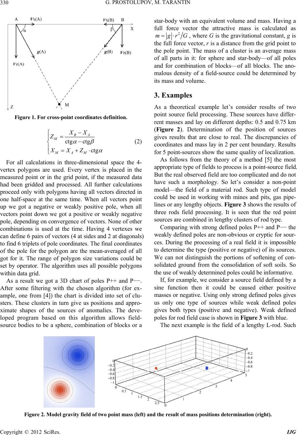

G. PROSTOLUPOV, M. TARANTIN

330

Figure 1. For cross-point coordinates definition.

g ctg

ctg



















(2)

For all calculations in three-dimensional space the 4-

vertex polygons are used. Every vertex is placed in the

measured point or in the grid point, if the measured data

had been gridded and processed. All further calculations

proceed only with polygons having all vectors directed in

one half-space at the same time. When all vectors point

up we got a negative or weakly positive pole, when all

vectors point down we got a positive or weakly negative

pole, depending on convergence of vectors. None of other

combinations is used at the time. Having 4 vertexes we

can define 6 pairs of vectors (4 at sides and 2 at diagonals)

to find 6 triplets of pole coordinates. The final coordinates

of the pole for the polygon are the mean-averaged of all

got for it. The range of polygon size variations could be

set by operator. The algorithm uses all possible polygons

within data grid.

As a result we got a 3D chart of poles P++ and P−−.

After some filtering with the chosen algorithm (for ex-

ample, one from [4]) the chart is divided into set of clu-

sters. These clusters in turn give us positions and appro-

ximate shapes of the sources of anomalies. The deve-

loped program based on this algorithm allows field-

source bodies to be a sphere, combination of blocks or a

star-body with an equivalent volume and mass. Having a

full force vector the attractive mass is calculated as

mgrG , where G is the gravitational constant, g is

the full force vector, r is a distance from the grid point to

the pole point. The mass of a cluster is an average mass

of all parts in it: for sphere and star-body—of all poles

and for combination of blocks—of all blocks. The ano-

malous density of a field-source could be determined by

its mass and volume.

3. Examples

As a theoretical example let’s consider results of two

point source field processing. These sources have differ-

rent masses and lay on different depths: 0.5 and 0.75 km

(Figure 2). Determination of the position of sources

gives results that are close to real. The discrepancies of

coordinates and mass lay in 2 per cent boundary. Results

for 5 point-sources show the same quality of localization.

As follows from the theory of a method [5] the most

appropriate type of fields to process is a point-source field.

But the real observed field are too complicated and do not

have such a morphology. So let’s consider a non-point

model—the field of a material rod. Such type of model

could be used in working with mines and pits, gas pipe-

lines or any lengthy objects. Figure 3 shows the results of

three rods field processing. It is seen that the red point

sources are combined in lengthy clusters of rod type.

Comparing with strong defined poles P++ and P−− the

weakly defined poles are non-obvious or cryptic for sour-

ces. During the processing of a real field it is impossible

to determine the type (positive or negative) of its sources.

We can not distinguish the portions of softening of con-

solidated ground from the consolidation of soft soils. So

the use of weakly determined poles could be informative.

If, for example, we consider a source field defined by a

sine function then it could be caused either positive

masses or negative. Using only strong defined poles gives

us only one type of sources while weak defined poles

gives both types (positive and negative). Weak defined

poles for rod field case is shown in Figure 3 with blue.

The next example is the field of a lengthy L-rod. Such

Figure 2. Model gravity field of two point mass (left) and the result of mass positions determination (right).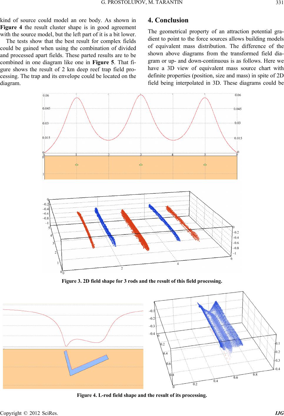

G. PROSTOLUPOV, M. TARANTIN 331

kind of source could model an ore body. As shown in

Figure 4 the result cluster shape is in good agreement

with the source model, but the left part of it is a bit lower.

The tests show that the best result for complex fields

could be gained when using the combination of divided

and processed apart fields. These parted results are to be

combined in one diagram like one in Figure 5. That fi-

gure shows the result of 2 km deep reef trap field pro-

cessing. The trap and its envelope could be located on the

diagram.

4. Conclusion

The geometrical property of an attraction potential gra-

dient to point to the force sources allows building models

of equivalent mass distribution. The difference of the

shown above diagrams from the transformed field dia-

gram or up- and down-continuous is as follows. Here we

have a 3D view of equivalent mass source chart with

definite properties (position, size and mass) in spite of 2D

field being interpolated in 3D. These diagrams could be

Figure 3. 2D field shape for 3 rod s an d the result of this field processin g .

Figure 4. L-rod field shape and the result of its p roces sing.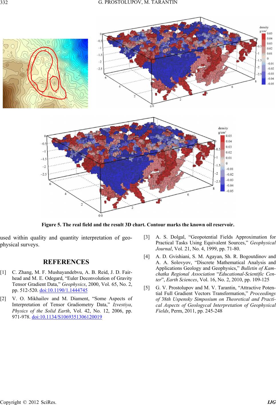

G. PROSTOLUPOV, M. TARANTIN

332

Figure 5. The real field and the result 3D chart. Contour marks the known oil reservoir.

used within quality and quantity interpretation of geo-

physical surveys.

REFERENCES

[1] C. Zhang, M. F. Mushayandebvu, A. B. Reid, J. D. Fair-

head and M. E. Odegard, “Euler Deconvolution of Gravity

Tensor Gradient Data,” Geophysics, 2000, Vol. 65, No. 2,

pp. 512-520. doi:10.1190/1.1444745

[2] V. O. Mikhailov and M. Diament, “Some Aspects of

Interpretation of Tensor Gradiometry Data,” Izvestiya,

Physics of the Solid Earth, Vol. 42, No. 12, 2006, pp.

971-978. doi:10.1134/S1069351306120019

[3] A. S. Dolgal, “Geopotential Fields Approximation for

Practical Tasks Using Equivalent Sources,” Geophysical

Journal, Vol. 21, No. 4, 1999, pp. 71-80.

[4] A. D. Gvishiani, S. M. Agayan, Sh. R. Bogoutdinov and

A. A. Solovyov, “Discrete Mathematical Analysis and

Applications Geology and Geophysics,” Bulletin of Kam-

chatka Regional Association “Educational-Scientific Cen-

ter”, Earth Sciences, Vol. 16, No. 2, 2010, pp. 109-125

[5] G. V. Prostolupov and M. V. Tarantin, “Attractive Poten-

tial Full Gradient Vectors Transformation,” Proceedings

of 38th Uspensky Simposium on Theoretical and Practi-

cal Aspects of Geologycal Interpretation of Geophysical

Fields, Perm, 2011, pp. 245-248