Lateral Stability Analysis of Heavy-Haul Vehicle on Curved Track Based on Wheel/Rail Coupled Dynamics

doi:10.4236/jtts.2012.22016

Paper Menu >>

Journal Menu >>

Journal of Transportation Technologies, 2012, 2, 150-157

http://dx.doi.org/10.4236/jtts.2012.22016 Published Online April 2012 (http://www.SciRP.org/journal/jtts)

Lateral Stability Analysis of Heavy-Haul Vehicle on

Curved Track Based on Wheel/Rail Coupled Dynamics

Kaiyun Wang, Pengfei Liu

Traction Power State Key Laboratory, Southwest Jiaotong University, Chengdu, China

Email: [email protected]

Received December 16, 2011; revised February 7, 2012; accepted March 1, 2012

ABSTRACT

Being viewed from the standpoint of whole system, the hunting stability of a heavy-haul railway vehicle on a curved

track is investigated in this paper. First, a model to simulate dynamic performance of the heavy-haul vehicle on the

elastic track is developed. Secondly, the reason of the hunting motion is analyzed, and a bifurcation diagram for the

vehicle on the curved track is put forward to simulate the nonlinear critical speed. Results show that the hunting motion

of the heavy-haul vehicle will appear due to the larger conicity, the initial lateral shift and the wheelset angle of attack.

With the hunting motion appearing, the lateral shift and force of the wheelset are changed sharply and periodically with

a wave of circa 3.6 m. There is obvious difference in the bifurcation diagram between on a curved track and on a tan-

gent track. Relative to the centerline of the track, each vehicle body on the curved track has two stable cycles. As for the

curved track with a radius of 600 m and a superelevation of 55 mm, the nonlinear critical speed of the heavy-haul vehi-

cle is 76.4 km/h.

Keywords: Hunting; Stability; Curved Track; Heavy-Haul Railway; Coupled Dynamics

1. Introduction

Developing heavy-haul railways is one efficient measure

to increase the transport volume. However, being re-

stricted to the landform in the heavy-haul railway, there

are many sharp curved tracks with the radius ranging

from 500 m to 1000 m. When a heavy-haul vehicle is

negotiating these curved tracks with low speeds, the phe-

nomenon of the hunting motion, usually taking place on

the tangent track, will also appear. Due to the hunting

motion on the curved tracks, the interaction force be-

tween the wheel and the rail is seriously enhanced, the

performance of the negotiation is severely deteriorated,

the rail is sharply worn, the rail life is clearly shortened,

and even the vehicle will derail on the curved track. So,

much attention should be paid to the vehicle hunting mo-

tion on the curved track.

Studies on the running stability of the railway vehicle

have been performed for almost half of century. The first

bifurcation analysis of the free running wheelset was

carried out by Huilgol [1] and in this research a hopf bi-

furcation from the steady state was revealed. The first

observation of chaotic oscillations in models of railway

vehicles was carried out by True et al. [2] and Petersen

[3]. Dukkipati [4] developed the mathematical linear

models to determine the lateral stability or hunting of

North American standard three-piece freight truck on

track/roller stands, and the theoretical model results were

compared with field test data performed by the Associa-

tion of American Railroads (AAR). In the meanwhile,

using linear models, a comparative study on the dynamic

stability and steady state curving behavior of some un-

conventional railway truck designs was carried out by

Dukkipati [5]. Further works demonstrating the hunting

stability of high-speed vehicle were carried out by Lee

and his team [6,7], including the stability on the tangent

track [6] and the stability on the curved track [7]. Lee et

al. [8] modeled eight degrees of freedom (DOFs) for

truck system moving on curved tracks, and it was re-

ported that the critical hunting speeds evaluated by using

the eight-DOF system differed significantly from those

done by the six-DOF system.

Unfortunately, up to now, there is little study about the

lateral stability of the heavy-haul vehicle on the curved

track, let alone the stability research based on the cou-

pled model between the vehicle and the track.

Therefore, being viewed from the standpoint of the

coupled system presented by Zhai et al. [9,10], investiga-

tion efforts will be focused on the nonlinear hunting sta-

bility of the heavy-haul vehicle on the curved track in

this paper. Firstly, a model to simulate the dynamic per-

formance of the heavy-haul vehicle on the elastic track is

established. Secondly, the reason of the hunting motion

on the curved track is analyzed. Lastly, a bifurcation dia-

K. Y. WANG ET AL. 151

gram for the vehicle on curved track is put forward to

simulate the nonlinear critical speed.

2. Dynamic Model of Heavy-Haul Vehicle on

Curved Track

A curved track contains three main elements such as ra-

dius, cant, and gauge. When a heavy-haul vehicle with

full freight passes through the small-radius curved track,

the interaction between the wheel and the rail is very

serious, as causes the track vibrating obviously. Figure 1

indicates a measured result [11] of dynamic gauge en-

largements on a small-radius curve track. It can be seen

from the Figure 1 that the dynamic gauge enlargement is

very clear and the maximum value is close to 3.5 mm.

Therefore, for an analysis on the vehicle dynamic per-

formance, including the stability on the curved track, it is

very necessary to take the dynamic vibration of the track

into account.

2.1. Coordinate Systems

The descriptions of the configuration and the orientation

of the railway vehicle on the track are related to the defi-

nition of coordinate systems. In order to describe the

absolute motion of the heavy-haul vehicle on a curved

track, two coordinate systems are needed: the inertial

coordinate system and the body fixed coordinate system.

Only taking a wheelset on a curved track for an example,

the coordinate systems are shown in Figure 2, where the

inertial coordinate system (Oi, Xi, Yi, Zi) is located on the

center line of the track and can not move with the

wheelset, and the wheelset fixed coordinate system (Ow,

Xw, Yw, Zw) is located in the mass center of the wheelset

and can move with the wheelset. In addition, the positive

directions of y in both systems are toward the inner rail

of the curved track or the right rail of the tangent track.

Relative to the inertial system, any of the vehicle body

has six DOFs, including three DOFs of transfer motions

in longitudinal (X), lateral (Y), and vertical (Z), three

45 50 55 60 65 70

Dynamic gauge enlargement (mm)

Speed (km/h)

Figure 1. Measured result of dynamic gauge enlargements

on the small-radius curve track.

Figure 2. Coordinate systems on curved track.

DOFs of a pitch motion (



), a rolling motion (



), and a

yaw motion (



). The absolute motion of the body of the

vehicle is the vector sum of the transfer and the rotation

motions. The relationship between the inertial system

and the body fixed system is shown in Figure 3 [12], in

which, p stands any point of a body, the vector rp (Oi, Xi,

Yi, Zi) in the inertial system stands for its static and spa-

tial position, the vector rp (OB, XB, YB, ZB) in the body

fixed system stands for its dynamic and spatial position

with respect to the inertial system,



rc is the transfer

vector in the body fixed system with respect to the iner-

tial system, and



ri is the absolute vector of a body.

So,



ri is calculated by:

icBpp



 Arr rr

(1)

in which, AB is the rotation matrix in the body fixed sys-

tem with respect to the inertial system and is formed as

following:

101

01 1







 







 



 

 



 



 





 

where,



is the angle difference of two coordinate sys-

tems caused by the superelevation (around X axis),



the angle difference of two coordinate systems (around Z

axis), in addition, these parameter values are determined

by the line type of the curved track.

According to the Equation (1), all the absolute vectors

of vehicle bodies can be calculated. If a body A and a

body B are conjoined by a suspension, the relative dis-

placement of the suspension points between A and B is

given by:

ABB A



 rrr (2)

in which, the



rA and



rB stand for the absolute vector of

body A and body B, respectively.

Therefore, the relative velocity of the suspension points

K. Y. WANG ET AL.

152

Figure 3. The vector of body with respect to the inertial

system.

between A and B is also given by:



AB t



 r

v (3)

If the stiffness matrix and the damping matrix in this

suspension are K and C, respectively, the force of the

suspension points is calculated as following:

AB AB

 FKr Cv (4)

2.2. Model of Heavy-Haul Vehicle

Figure 4 shows a three-piece structure of a heavy-haul

vehicle which includes two side frames and one bolster.

Nowadays, the three-piece structure is widely applied in

the heavy-haul vehicle in CR. In order to reduce the un-

sprung mass, the elastic rubber is set in the axle-box, as

is the primary suspension. Apart from this, the compo-

nents of the structure are similar to those introduced by

Xia [13].

The vehicle is modeled as a multi-body dynamic sys-

tem, as is shown in Figure 5. In Figure 5, Z, Y and Φ

denote the DOFs of vertical, lateral and roll motions of a

component; subscripts c, t and w represent carbody, side

frame and wheelset; subscripts L and R denote the left

and right side respectively; Ksz and Csz are the vertical

stiffness and damping of the secondary suspension; Ksy

and Csy are the lateral stiffness and damping of the sec-

ondary suspension; Kpz and Cpz are the vertical stiffness

and damping of the primary suspension; and Kpy and Cpy

are the lateral stiffness and damping of the primary sus-

pension.

There are eleven principal components, including one

carbody, two bolsters, four side frames, and four wheel-

sets. It is shown that the carbody is connected to the bol-

ster via the center plates modeled as a spherical joint.

Because the radius of the spherical joint is small com-

pared with the other dimensions of the carbody, and the

effect of the friction produced by the spherical joint on

the roll rotation of the carbody and the bolster is ne-

glected. But the effect of the friction torque on the yaw

rotation is still considered. In the secondary suspension,

the bolsters are elastically connected to the side frames

by springs vertically, and a one-dimension model without

Centerplate

Whee

Axl e

Primary suspension

Secondary suspension

Side frame

Bolster

Figure 4. The construction of the he avy-haul vehicle in CR.

YtL

ZtL

Ksy

syK

szC

szYtR

ZtR

Cpy

Kpz

Cpz

Figure 5. Description of heavy-haul vehicle dynamics model

with end view.

stick mode is applied to simulate the dry friction in the

wedge damper system. The primary suspension is mod-

eled as the parameters of Kp and Cp in longitudinal, lat-

eral and vertical.

All of components are assumed to be rigid. The DOFs

of a heavy-haul vehicle are given in Table 1, where the

total DOFs are 47.

2.3. Model of Track

A five-parameter model [9,10] is adopted to model the

railway track, as is shown in Figure 6. The rail is mod-

eled as a Bernoulli-Euler beam discretely supported at

masses. The three layers of discrete springs and dampers

represent the elasticity and damping effects of the rail

fastening, the ballast, and the subgrade respectively.

2.4. Model of the Wheel-Rail Contact

The wheelsets provide the supports for the entire vehicle

and supply the contact forces that keep the vehicle sys-

tem on the track. A new model of three-dimensional

geometrical contact between wheel and rail [10,14] is

K. Y. WANG ET AL. 153

Table 1. DOFs of a heavy-haul vehicle.

Component Long. Lat. Vert. Roll Pitch Yaw

Carbody - Yc Zc







Bolster

(i = 1, 2) - - - - -



Front side frame

(i = 1, 2) XtFi YtFi ZtFi -



tFi



tFi

Rear side frame

(i = 1, 2) XtRi YtRi ZtRi -



tRi



tRi

Wheelset

(i = 1 - 4) - Ywi Zwi







Figure 6. Description of a five-parameter track model.

adopted. All the contact parameters are calculated online,

including the contact point and its curvature, the conicity,

and so on. The normal force of wheel-rail contact is de-

scribed by a non-linear Hertzian contact theory, and the

tangential force is calculated by a Shen-Hedrick-Elkins

formula [15].

3. Reason of Hunting Motion of Heavy-Haul

Vehicle on Curved Track

When a heavy-haul vehicle negotiates a curved track at a

low speed, some unbalanced centrifugal forces will ap-

pear in the vehicle system due to the multiple effects

such as speed, curve radius, superelevation, and so on.

Under the action of the unbalanced centrifugal forces,

wheelsets will deviate from the track centerline. Both the

theoretical and experimental results [11] show that the

lateral shifts of wheelsets are bigger than 4 mm usually.

Figure 7 illustrates the theoretical result of the conic-

ity for the wheel tread of LM and the rail profile of the

heavy-haul railway. During the curved negotiation, the

lateral shifts of wheelsets are bigger than 4 mm. So the

conicity value is more than 0.1, as can help to improve

the self-steering ability of the wheelset. It is worth point-

ing out that the conicity value of the curved track is big-

ger than the value of the tangent track. In addition, as for

the vehicle system on the curved track, the lateral shift is

a kind of outside excitation, and the wheelset centerline

is not under the radial situation, and the wheelset angle of

attack, i.e. the angle between the wheelset axis and the

radius of the curve, will appear on the wheelset.

Consequently, under the effects of the large conicity,

Figure 7. Conicity versus lateral shift of wheelset.

the excitation of the lateral shift, and the wheelset angle

of attack, the hunting motion appears easily for the

wheelsets of a heavy-haul vehicle. Especially for the

wagons assembled with the worn components and the

worsened suspensions, the hunting stability on curved

track is much worse.

Furthermore, a numerical example of the hunting mo-

tion of a heavy-haul vehicle with no freight is given, in

which, the radius is 600 m, the superelevation of outer

rail is 55 mm, the negotiation speed is 85 km/h, the tran-

sitions are made of parabolic curves, and other dynamic

parameters are evaluated [10,16]. The calculated results

of the lateral shift of the wheelset are presented in Figure

8, including the time and frequency domain results. It can

be seen from Figure 8(a) that the phenomenon of the

hunting motion appears at the point of spiral to curve, at

the point of curve to spiral, and in the whole circular line,

and there is lateral and periodic oscillation on the wheel-

set. Under this situation of the hunting motion, the

dominant frequency of the lateral shift is circa 6.5 Hz, as

is shown in Figure 8(b).

According to the following formula





(5)

in which,



stands the wave length, v is the vehicle speed,

and f is the dominant frequency.

So, the hunting wave length is circa 3.6 m corre-

spondingly, which is quite close to the hunting wave

length on a tangent track [17].

Figure 9 shows the calculated results of the wheelset

lateral force under this condition of the hunting motion.

It is noticeable that the lateral interaction forces between

the wheel and the rail change severely and fluctuate pe-

riodically when the phenomenon of the hunting motion

of the wheelset appears. The main reason is that, due to

the effects of the lateral shift and wheelset angle of attack,

the severe impact contact may happen between the root

of the wheel flange and the rail side.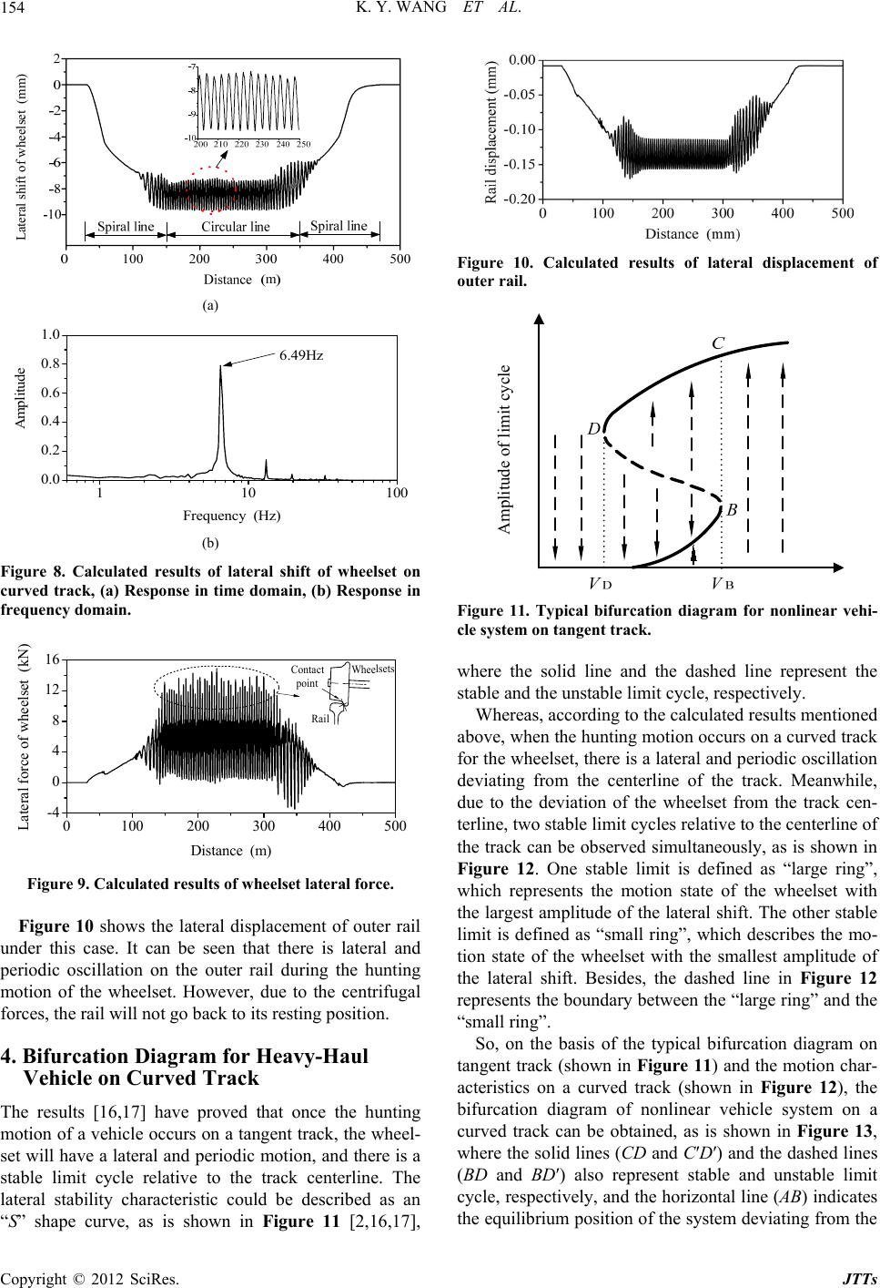

K. Y. WANG ET AL.

154

Lateral shift of wheelset (mm)

(a)

110

0.0

0.2

0.4

0.6

0.8

1.0

100

Amplitude

Frequency (Hz)

6.49Hz

(b)

Figure 8. Calculated results of lateral shift of wheelset on

curved track, (a) Response in time domain, (b) Response in

frequency domain.

0100 200 300400 500

-4

Wheelsets

Rail

Contact

point

Lateral force of wheelset (kN)

Distance (m)

Figure 9. Calculated results of wheelset lateral force.

Figure 10 shows the lateral displacement of outer rail

under this case. It can be seen that there is lateral and

periodic oscillation on the outer rail during the hunting

motion of the wheelset. However, due to the centrifugal

forces, the rail will not go back to its resting position.

4. Bifurcation Diagram for Heavy-Haul

Vehicle on Curved Track

The results [16,17] have proved that once the hunting

motion of a vehicle occurs on a tangent track, the wheel-

set will have a lateral and periodic motion, and there is a

stable limit cycle relative to the track centerline. The

lateral stability characteristic could be described as an

“S” shape curve, as is shown in Figure 11 [2,16,17],

Figure 10. Calculated results of lateral displacement of

outer rail.

Amplitude of limit cycle

Figure 11. Typical bifurcation diagram for nonlinear vehi-

cle system on tangent track.

where the solid line and the dashed line represent the

stable and the unstable limit cycle, respectively.

Whereas, according to the calculated results mentioned

above, when the hunting motion occurs on a curved track

for the wheelset, there is a lateral and periodic oscillation

deviating from the centerline of the track. Meanwhile,

due to the deviation of the wheelset from the track cen-

terline, two stable limit cycles relative to the centerline of

the track can be observed simultaneously, as is shown in

Figure 12. One stable limit is defined as “large ring”,

which represents the motion state of the wheelset with

the largest amplitude of the lateral shift. The other stable

limit is defined as “small ring”, which describes the mo-

tion state of the wheelset with the smallest amplitude of

the lateral shift. Besides, the dashed line in Figure 12

represents the boundary between the “large ring” and the

“small ring”.

So, on the basis of the typical bifurcation diagram on

tangent track (shown in Figure 11) and the motion char-

acteristics on a curved track (shown in Figure 12), the

bifurcation diagram of nonlinear vehicle system on a

curved track can be obtained, as is shown in Figure 13,

where the solid lines (CD and C′D′) and the dashed lines

(BD and BD′) also represent stable and unstable limit

cycle, respectively, and the horizontal line (AB) indicates

the equilibrium position of the system deviating from the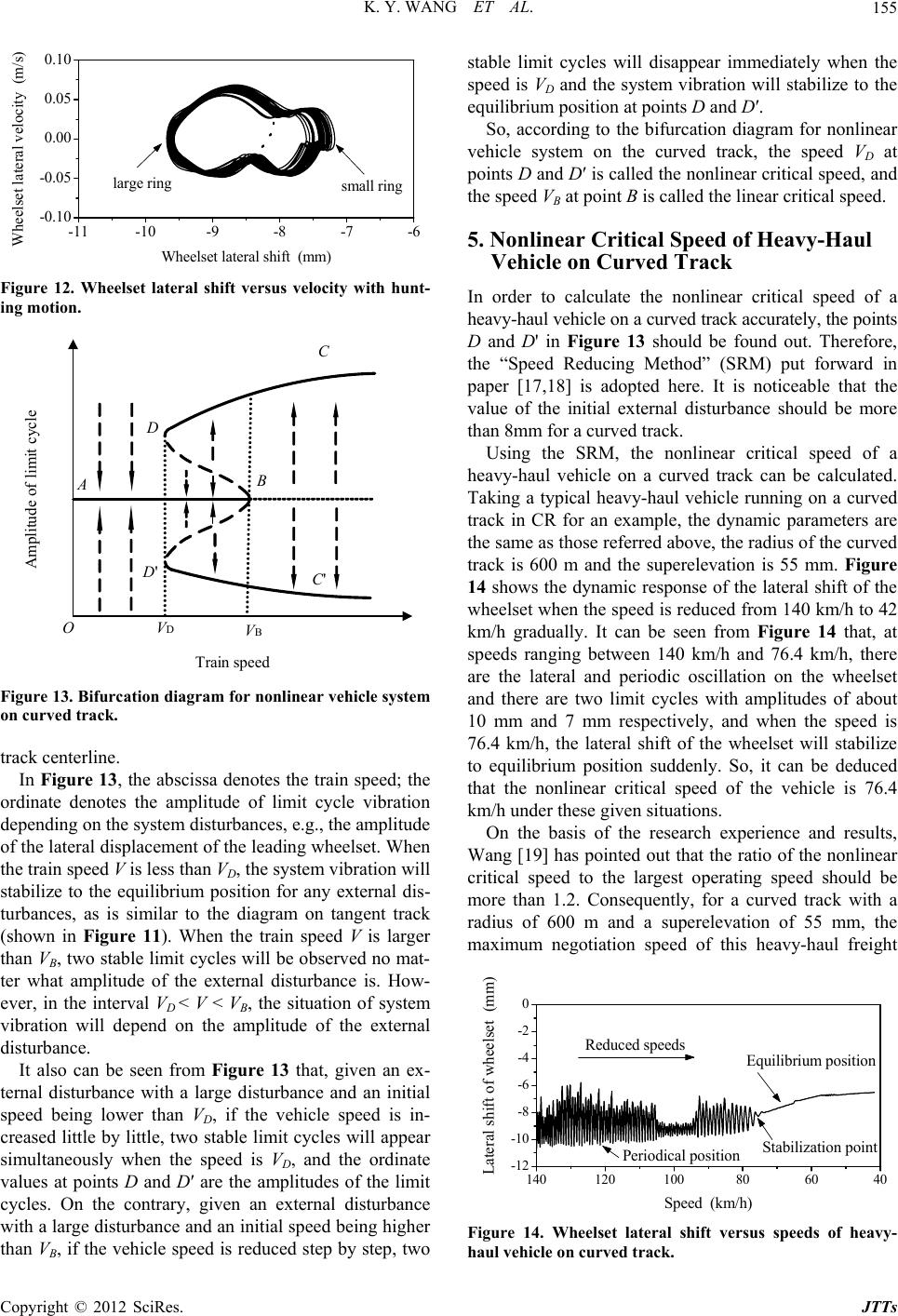

K. Y. WANG ET AL. 155

-11-10-9-8-7 -6

-0.10

-0.05

0.00

0.05

0.10

small ring

Wheelset lateral velocity (m/s)

Wheelset lateral shift (mm)

large ring

Figure 12. Wheelset lateral shift versus velocity with hunt-

ing motion.

VDVB

Amplitude of limit cycle

Train speed

Figure 13. Bifurcation diagram for nonlinear vehicle system

on curved track.

track centerline.

In Figure 13, the abscissa denotes the train speed; the

ordinate denotes the amplitude of limit cycle vibration

depending on the system disturbances, e.g., the amplitude

of the lateral displacement of the leading wheelset. When

the train speed V is less than VD, the system vibration will

stabilize to the equilibrium position for any external dis-

turbances, as is similar to the diagram on tangent track

(shown in Figure 11). When the train speed V is larger

than VB, two stable limit cycles will be observed no mat-

ter what amplitude of the external disturbance is. How-

ever, in the interval VD < V < VB, the situation of system

vibration will depend on the amplitude of the external

disturbance.

It also can be seen from Figure 13 that, given an ex-

ternal disturbance with a large disturbance and an initial

speed being lower than VD, if the vehicle speed is in-

creased little by little, two stable limit cycles will appear

simultaneously when the speed is VD, and the ordinate

values at points D and D′ are the amplitudes of the limit

cycles. On the contrary, given an external disturbance

with a large disturbance and an initial speed being higher

than VB, if the vehicle speed is reduced step by step, two

stable limit cycles will disappear immediately when the

speed is VD and the system vibration will stabilize to the

equilibrium position at points D and D′.

So, according to the bifurcation diagram for nonlinear

vehicle system on the curved track, the speed VD at

points D and D′ is called the nonlinear critical speed, and

the speed VB at point B is called the linear critical speed.

5. Nonlinear Critical Speed of Heavy-Haul

Vehicle on Curved Track

In order to calculate the nonlinear critical speed of a

heavy-haul vehicle on a curved track accurately, the points

D and D' in Figure 13 should be found out. Therefore,

the “Speed Reducing Method” (SRM) put forward in

paper [17,18] is adopted here. It is noticeable that the

value of the initial external disturbance should be more

than 8mm for a curved track.

Using the SRM, the nonlinear critical speed of a

heavy-haul vehicle on a curved track can be calculated.

Taking a typical heavy-haul vehicle running on a curved

track in CR for an example, the dynamic parameters are

the same as those referred above, the radius of the curved

track is 600 m and the superelevation is 55 mm. Figure

14 shows the dynamic response of the lateral shift of the

wheelset when the speed is reduced from 140 km/h to 42

km/h gradually. It can be seen from Figure 14 that, at

speeds ranging between 140 km/h and 76.4 km/h, there

are the lateral and periodic oscillation on the wheelset

and there are two limit cycles with amplitudes of about

10 mm and 7 mm respectively, and when the speed is

76.4 km/h, the lateral shift of the wheelset will stabilize

to equilibrium position suddenly. So, it can be deduced

that the nonlinear critical speed of the vehicle is 76.4

km/h under these given situations.

On the basis of the research experience and results,

Wang [19] has pointed out that the ratio of the nonlinear

critical speed to the largest operating speed should be

more than 1.2. Consequently, for a curved track with a

radius of 600 m and a superelevation of 55 mm, the

maximum negotiation speed of this heavy-haul freight

140 120 10080604

-12

-10

-8

-6

-4

-2

Stabilization point

Equilibrium position

Reduced speeds

Lateral shift of wheelset (mm)

eed

(

km/h

)

Periodical position

Figure 14. Wheelset lateral shift versus speeds of heavy-

haul vehicle on curved track.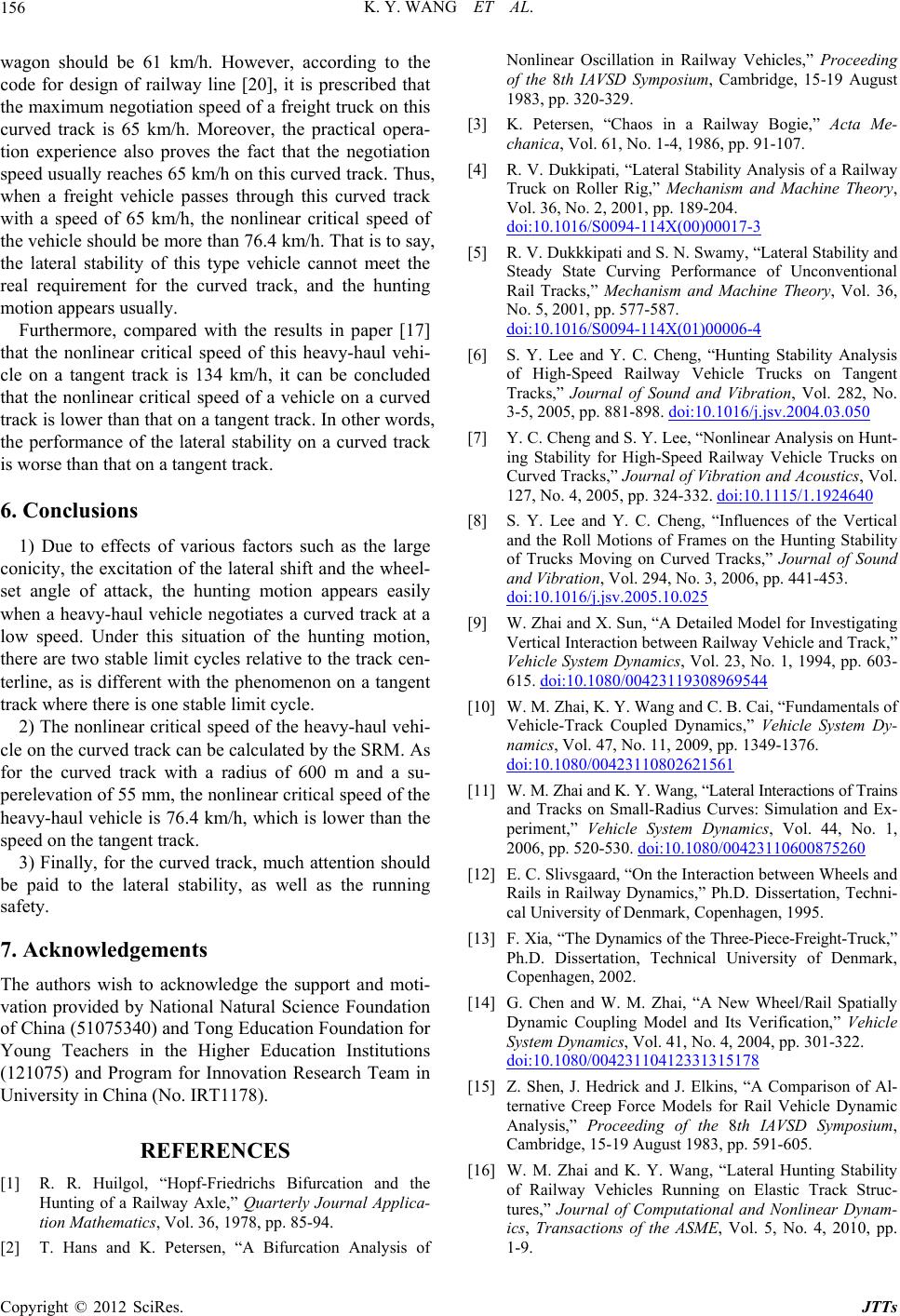

K. Y. WANG ET AL.

156

wagon should be 61 km/h. However, according to the

code for design of railway line [20], it is prescribed that

the maximum negotiation speed of a freight truck on this

curved track is 65 km/h. Moreover, the practical opera-

tion experience also proves the fact that the negotiation

speed usually reaches 65 km/h on this curved track. Thus,

when a freight vehicle passes through this curved track

with a speed of 65 km/h, the nonlinear critical speed of

the vehicle should be more than 76.4 km/h. That is to say,

the lateral stability of this type vehicle cannot meet the

real requirement for the curved track, and the hunting

motion appears usually.

Furthermore, compared with the results in paper [17]

that the nonlinear critical speed of this heavy-haul vehi-

cle on a tangent track is 134 km/h, it can be concluded

that the nonlinear critical speed of a vehicle on a curved

track is lower than that on a tangent track. In other words,

the performance of the lateral stability on a curved track

is worse than that on a tangent track.

6. Conclusions

1) Due to effects of various factors such as the large

conicity, the excitation of the lateral shift and the wheel-

set angle of attack, the hunting motion appears easily

when a heavy-haul vehicle negotiates a curved track at a

low speed. Under this situation of the hunting motion,

there are two stable limit cycles relative to the track cen-

terline, as is different with the phenomenon on a tangent

track where there is one stable limit cycle.

2) The nonlinear critical speed of the heavy-haul vehi-

cle on the curved track can be calculated by the SRM. As

for the curved track with a radius of 600 m and a su-

perelevation of 55 mm, the nonlinear critical speed of the

heavy-haul vehicle is 76.4 km/h, which is lower than the

speed on the tangent track.

3) Finally, for the curved track, much attention should

be paid to the lateral stability, as well as the running

safety.

7. Acknowledgements

The authors wish to acknowledge the support and moti-

vation provided by National Natural Science Foundation

of China (51075340) and Tong Education Foundation for

Young Teachers in the Higher Education Institutions

(121075) and Program for Innovation Research Team in

University in China (No. IRT1178).

REFERENCES

[1] R. R. Huilgol, “Hopf-Friedrichs Bifurcation and the

Hunting of a Railway Axle,” Quarterly Journal Applica-

tion Mathematics, Vol. 36, 1978, pp. 85-94.

[2] T. Hans and K. Petersen, “A Bifurcation Analysis of

Nonlinear Oscillation in Railway Vehicles,” Proceeding

of the 8th IAVSD Symposium, Cambridge, 15-19 August

1983, pp. 320-329.

[3] K. Petersen, “Chaos in a Railway Bogie,” Acta Me-

chanica, Vol. 61, No. 1-4, 1986, pp. 91-107.

[4] R. V. Dukkipati, “Lateral Stability Analysis of a Railway

Truck on Roller Rig,” Mechanism and Machine Theory,

Vol. 36, No. 2, 2001, pp. 189-204.

doi:10.1016/S0094-114X(00)00017-3

[5] R. V. Dukkkipati and S. N. Swamy, “Lateral Stability and

Steady State Curving Performance of Unconventional

Rail Tracks,” Mechanism and Machine Theory, Vol. 36,

No. 5, 2001, pp. 577-587.

doi:10.1016/S0094-114X(01)00006-4

[6] S. Y. Lee and Y. C. Cheng, “Hunting Stability Analysis

of High-Speed Railway Vehicle Trucks on Tangent

Tracks,” Journal of Sound and Vibration, Vol. 282, No.

3-5, 2005, pp. 881-898. doi:10.1016/j.jsv.2004.03.050

[7] Y. C. Cheng and S. Y. Lee, “Nonlinear Analysis on Hunt-

ing Stability for High-Speed Railway Vehicle Trucks on

Curved Tracks,” Journal of Vibration and Acoustics, Vol.

127, No. 4, 2005, pp. 324-332. doi:10.1115/1.1924640

[8] S. Y. Lee and Y. C. Cheng, “Influences of the Vertical

and the Roll Motions of Frames on the Hunting Stability

of Trucks Moving on Curved Tracks,” Journal of Sound

and Vibration, Vol. 294, No. 3, 2006, pp. 441-453.

doi:10.1016/j.jsv.2005.10.025

[9] W. Zhai and X. Sun, “A Detailed Model for Investigating

Vertical Interaction between Railway Vehicle and Track,”

Vehicle System Dynamics, Vol. 23, No. 1, 1994, pp. 603-

615. doi:10.1080/00423119308969544

[10] W. M. Zhai, K. Y. Wang and C. B. Cai, “Fundamentals of

Vehicle-Track Coupled Dynamics,” Vehicle System Dy-

namics, Vol. 47, No. 11, 2009, pp. 1349-1376.

doi:10.1080/00423110802621561

[11] W. M. Zhai and K. Y. Wang, “Lateral Interactions of Trains

and Tracks on Small-Radius Curves: Simulation and Ex-

periment,” Vehicle System Dynamics, Vol. 44, No. 1,

2006, pp. 520-530. doi:10.1080/00423110600875260

[12] E. C. Slivsgaard, “On the Interaction between Wheels and

Rails in Railway Dynamics,” Ph.D. Dissertation, Techni-

cal University of Denmark, Copenhagen, 1995.

[13] F. Xia, “The Dynamics of the Three-Piece-Freight-Truck,”

Ph.D. Dissertation, Technical University of Denmark,

Copenhagen, 2002.

[14] G. Chen and W. M. Zhai, “A New Wheel/Rail Spatially

Dynamic Coupling Model and Its Verification,” Vehicle

System Dynamics, Vol. 41, No. 4, 2004, pp. 301-322.

doi:10.1080/00423110412331315178

[15] Z. Shen, J. Hedrick and J. Elkins, “A Comparison of Al-

ternative Creep Force Models for Rail Vehicle Dynamic

Analysis,” Proceeding of the 8th IAVSD Symposium,

Cambridge, 15-19 August 1983, pp. 591-605.

[16] W. M. Zhai and K. Y. Wang, “Lateral Hunting Stability

of Railway Vehicles Running on Elastic Track Struc-

tures,” Journal of Computational and Nonlinear Dynam-

ics, Transactions of the ASME, Vol. 5, No. 4, 2010, pp.

1-9.

K. Y. WANG ET AL.

157

[17] K. Y. Wang and P. F. Liu, “Characteristic of Dynamic

Interaction between Wheel and Rail Due to the Hunting

Motion on Heavy-Haul Railway,” Engineering Mechan-

ics, Vol. 28, No. 1, 2012, pp. 235-239.

[18] P. B. Wu and J. Zeng, “A New Method to Determine

Linear and Nonlinear Critical Speed of the Vehicle Sys-

tem,” Rolling and Stock, Vol. 38, No. 5, 2000, pp. 1-4.

[19] F. T. Wang, “Vehicle System Dynamics,” China Railway

Press, Beijing, 1994.

[20] GB50090-2006, “Code for Design of Railway Line,”

China Planning Press, Beijing, 2006.