Reliability Analysis of Systems Based on the UFLP under Facility Failure and Conditional Supply Cases

doi:10.4236/apm.2012.22019

Paper Menu >>

Journal Menu >>

Advances in Pure Mathematics, 2012, 2, 128-132

http://dx.doi.org/10.4236/apm.2012.22019 Published Online March 2012 (http://www.SciRP.org/journal/apm)

Reliability Analysis of Systems Based on the UFLP under

Facility Failure and Conditional Supply Cases

Min Wang, Zongtian Wei, Yun He

Department of Mathematics, Xi’an University of Architecture and Technology, Xi’an, China

Email: [email protected]

Received November 24, 2011; revised January 10, 2012; accepted January 20, 2012

ABSTRACT

The reliability of facility location problems has been received wide attention for several decades. Researchers formulate

varied models to optimize the reliability of location decisions. But the most of such studies are not practical since the

models are too ideal. In this paper, based on the classical uncapacitated fixed-charge location problem (UFLP) and

some supply constraints from the reality, we distinguish deterministic facility failure and stochastic facility failure cases

to formulate models to measure the reliability of a system. The computational results and reliability envelopes for a

specific example are also given.

Keywords: Reliability Analysis; Facility Failure; Supply Constraint; Uncap acitated Fixed Charge Location Problem

1. Introduction

The uncapacitated fixed-ch arge location problem (UFLP)

[1] is a classical facility location problem that chooses

facility locations and assignments of customers to facili-

ties to minimize th e sum of fixed and transpor tation costs.

Once a set of facilities has been constructed, however,

one or more of them may from time to time become un-

available, we call it the facility failure. For ex ample, due

to inclement weather, earthquakes, sabotage, or changes

in ownership. The facility “failures” may result in exces-

sive transportation costs as customers previously served

by these facilities must now be served by more distant

ones. Snyder and Daskin [2] define the “reliability” of a

system as the ability of a system to perform well even

when parts of the system have failed. They formulate

models based on the UFLP and other classical discrete

location problems to optimize the reliability of a system.

However, they ignore an actual situation that suppliers

would not like to serve the customers too far from them

when the supplier who serves these customers previously

has failed.

Throughout this pa per, we use the concept “reliab ility”

defined in [2]. In this paper, ad opting th e facility locatio n

analysis framework, we consider facility systems’ reli-

ability analysis based on the UFLP and some supply cons-

traints when subject to facility failu res.

The remainder of this paper is structured as follows.

We formulate two reliability analysis models based on

the UFLP in§2. The computational results and the reli-

ability envelops of an example are presented in§3. In§4,

we give a summary of this paper.

2. Models

The facility location problem is a classical optimization

problem to determine the number and locations of a set

of facilities and assign customers to these in such a way

that the total cost is minimized. Two types of costs are

considered in the problem. A setup cost (facility cost) oc-

curs while a facility is opened, and a connection cost

occurs while a customer is assigned to the opened facility.

A fruitful research results have obtained in this field and

the topic remain hot still (see [3-6] and the references

therein).

2.1. The Uncapacitated Fixed-Charge Location

Problem

If an arbitrary number of customers can be connected to

a facility, the problem is called UFLP. The follows is th e

model of the classical facility location problem UFLP.

Sets:

: set of customers, indexed by ; i

: set of potential facility locations, indexed by . j

hiI

Parameters:

: demand at customer ;

: fixed cost of open a facility at ;

jJ

dij

c: the distance from customer to facility ;

: transportation cost per un it per distance;

: weight of the fixed cost in the objective function.



Decision variables: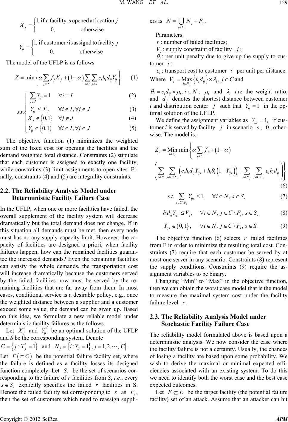

M. WANG ET AL. 129

1,ifa facilityisopened

0, ot

X





atlocation

herwise

dtofacility

herwise

1, if customerisassign

0, ot

Y





The model of the UFLP is as follows



min 1

jJi iiijij

IjJ









chdY













(2)

(3)

(4 )

(5)

(1)









.. 0, 1

0,1 ,

ij j

YiI

YX iIjJ

st XjJ

YiIjJ























The objective function (1) minimizes the weighted

sum of the fixed cost for opening the facilities and the

demand weighted total distance. Constraints (2) stipulate

that each customer is assigned to exactly one facility,

while constraints (3) limit assignments to open sites. Fi-

nally, constraints (4) and (5) are integrality co nstraints.

2.2. The Reliability Analysis Model under

Deterministic Facility Failure Case

In the UFLP, when o ne or mo re facilities have failed, the

overall supplement of the facility system will decrease

dramatically but the total demand does not change. If in

this situation all demands must be met, then every node

must has no any supply capacity limit. However, the ca-

pacity of facilities are designed a priori, when facility

failures happen, how can the remained facilities guaran-

tee the increased demands? Even the remaining facilities

can satisfy the whole demands, the transportation cost

will increase dramatically because the customers served

by the failed facilities now must be served by the re-

maining facilities that are far away from them. In most

cases, conditional service is a desirable policy, e.g., once

the weighted distance between a supplier and a customer

exceed some value, the demand can be given up. Based

on this idea, we formulate a new reliable model under

deterministic facility failures as the follows.

Let

and ij

Y be an optimal solution of the UFLP

and S be the corresponding system. Denote

C:



jX



and :1

jij

NiY



,1,2,,.j C

Let

C be the potential failure facility set, where

the failure is defined as a facility losses its designed

function completely. Let r be the set of scenarios cor-

responding to the failure of r facilities from S, i.e., every

Sr explicitly specifies the failed facilities in S.

Denote the failed facility set corresponding to

then the set of customers which need to reassign suppli-

ers is

NNF









Parameters:

: number of failed facilities;

: supply constraint of facility ;



: per unit penalty due to give up the supply to cus-

tomer ;

c i: transport cost to customer per unit per distance.





Max ,

jiiji

VhdjC





Where





,cdi N

and

iiiji



, i



and i





are the weight ratio,

and ij denotes the shortest distance between customer

i and distribution center such that Y in the op-

timal solution of the UFLP.

dj1

ij 

We define the assignment variables as ijs



if cus-

tomer i is served by facility jin scenario

, ,



0other-

wise. The model is:



Min min1

sjs

sS jC

i iij ijsi iijsi iij

iNjCFiN jCF

chd YhYchd







 































 

..1, ,

ijs r

jCF

(6)

tY iNsS







(7)

,,\,

iij ijsjsr

hd YViNjCFsS (8)



 





0,1 ,,\,

ijss r

YiNjCFsS (9)



 

The objective function (6) selects failed facilities

from F in order to minimize the resulting total cost. Con-

straints (7) require that each customer be served by at

most one server in any scenario. Constraints (8) represent

the supply conditions. Constraints (9) require the as-

signment variables to be binary.

Changing “Min” to “Max” in the objective function,

then we can obtain the worst case model that is the model

to measure the maximal system cost under the facility

failure level .

2.3. The Reliability Analysis Model under

Stochastic Facility Failure Case

The reliability model formulated above is based upon a

deterministic analysis. We now consider the case where

the facility failure is not a certainty. Usually, the chances

of losing a facility are based upon some probability. We

wish to derive the maximal or minimal expected effi-

ciencies associated with an existing system. To do this

we need to identify both the worst case and the best case

expected outcome s.

Let E be the target facility (the potential failure

facility) set of an attack. Assume that an attacker can hit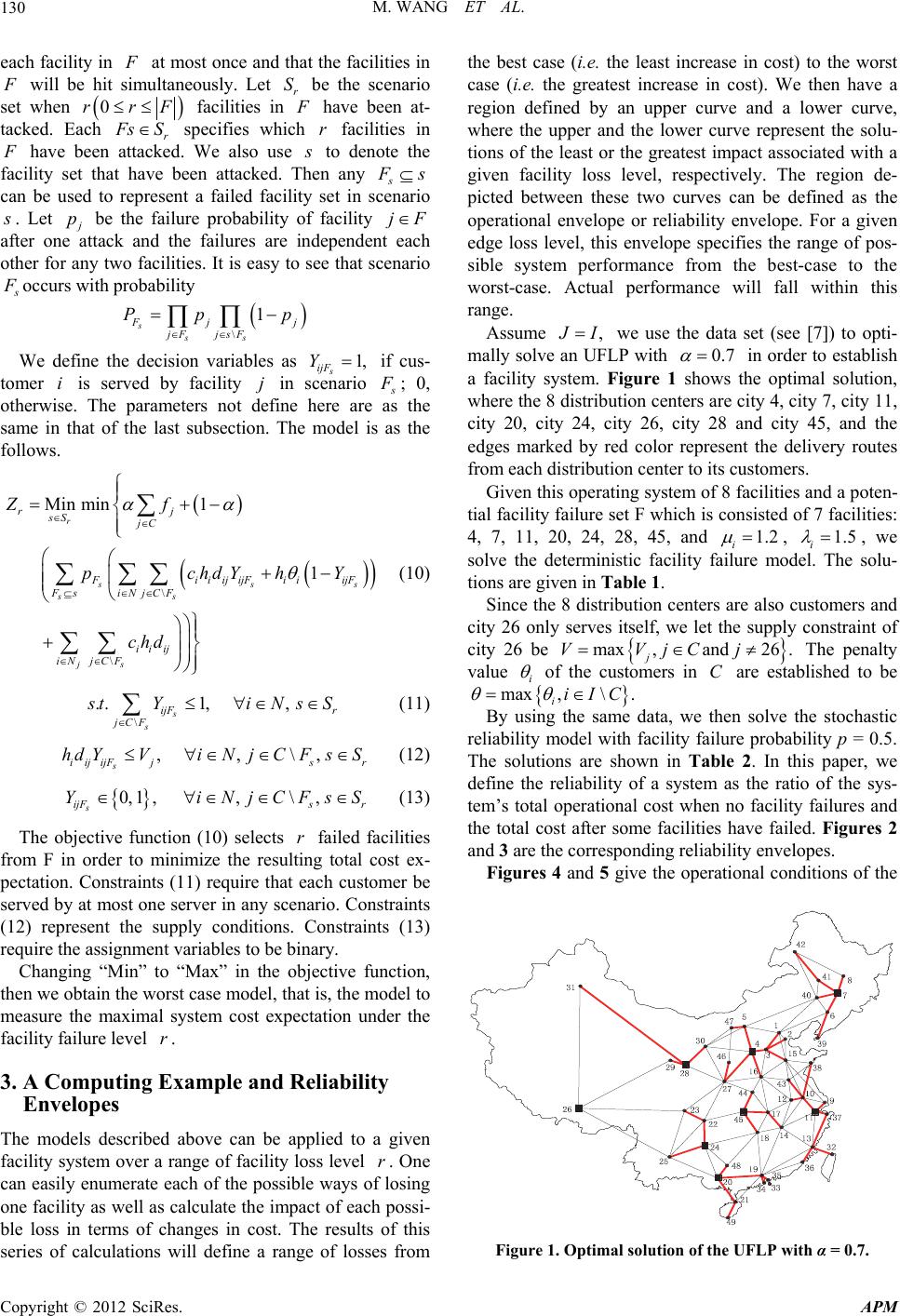

M. WANG ET AL.

130

at most once and that the facilities in each facility in

will be hit simultaneously. Let be the scenario

set when r



0rrF facilities in

have been at-

tacked. Each r

sSr specifies which facilities in

have been attacked. We also use

to denote the

facility set that have been attacked. Then any s

s

can be used to represent a failed facility set in scenario

. Let

p be the failure probability of facility jF



after one attack and the failures are independent each

other for any two facilities. It is easy to see that scenario

occurs with probability



p

jF j



1,

We define the decision variables as s

ijF if cus-

tomer is served by facility in scenario

i j

; 0,

otherwise. The parameters not define here are as the

same in that of the last subsection. The model is as the

follows.





min

FijF ijF

iNjCF

iiij

jCF

h Y

chd









































i i

dYh







Min











i i













(10)

.. s

ijF

jCF





iNs

C F

\ ,

Nj

S

s S

CFsS

(11)

j ijFj

Y Vj



0,1 ,,

i i

ijF

i

Yi

N (12)

s (13)

The objective function (10) selects failed facilities

from F in order to minimize the resulting total cost ex-

pectation. Constraints (11) require that each customer be

served by at most one server in any scenario. Constraints

(12) represent the supply conditions. Constraints (13)

require the assignment variables to be binary.

Changing “Min” to “Max” in the objective function,

then we obtain the worst case model, that is, the model to

measure the maximal system cost expectation under the

facility failure level .

3. A Computing Example and Reliability

Envelopes

The models described above can be applied to a given

facility system over a range of facility loss level . One

can easily enumerate each of the possible ways of losing

one facility as well as calculate the impact of each possi-

ble loss in terms of changes in cost. The results of this

series of calculations will define a range of losses from

the best case (i.e. the least increase in cost) to the worst

case (i.e. the greatest increase in cost). We then have a

region defined by an upper curve and a lower curve,

where the upper and the lower curve represent the solu-

tions of the least or the greatest impact associated with a

given facility loss level, respectively. The region de-

picted between these two curves can be defined as the

operational envelope or reliability envelope. For a given

edge loss level, this envelope specifies the range of pos-

sible system performance from the best-case to the

worst-case. Actual performance will fall within this

range.

Assume



we use the data set (see [7]) to opti-

mally solve an UFLP with 0.7





1.2

in order to establish

a facility system. Figure 1 shows the optimal solution,

where the 8 distribution centers are city 4, city 7, city 11,

city 20, city 24, city 26, city 28 and city 45, and the

edges marked by red color represent the delivery routes

from each distribution center to its customers.

Given this operating system of 8 facilities and a poten-

tial facility failure set F which is consisted of 7 facilities:

4, 7, 11, 20, 24, 28, 45, and i1.5, i







, we

solve the deterministic facility failure model. The solu-

tions are given in Table 1.

Since the 8 distribution centers are also customers and

city 26 only serves itself, we let the supply constraint of

city 26 be





max,and26.VVjCj

j The penalty

value



of the customers in are established to be C





max ,\ .iIC





By using the same data, we then solve the stochastic

reliability model with facility failure probability p = 0.5.

The solutions are shown in Table 2. In this paper, we

define the reliability of a system as the ratio of the sys-

tem’s total operational cost when no facility failures and

the total cost after some facilities have failed. Figures 2

and 3 are the corresponding reliability envelopes.

Figures 4 and 5 give the operational conditions of the

Figure 1. Optimal solution of the UFLP with α = 0.7.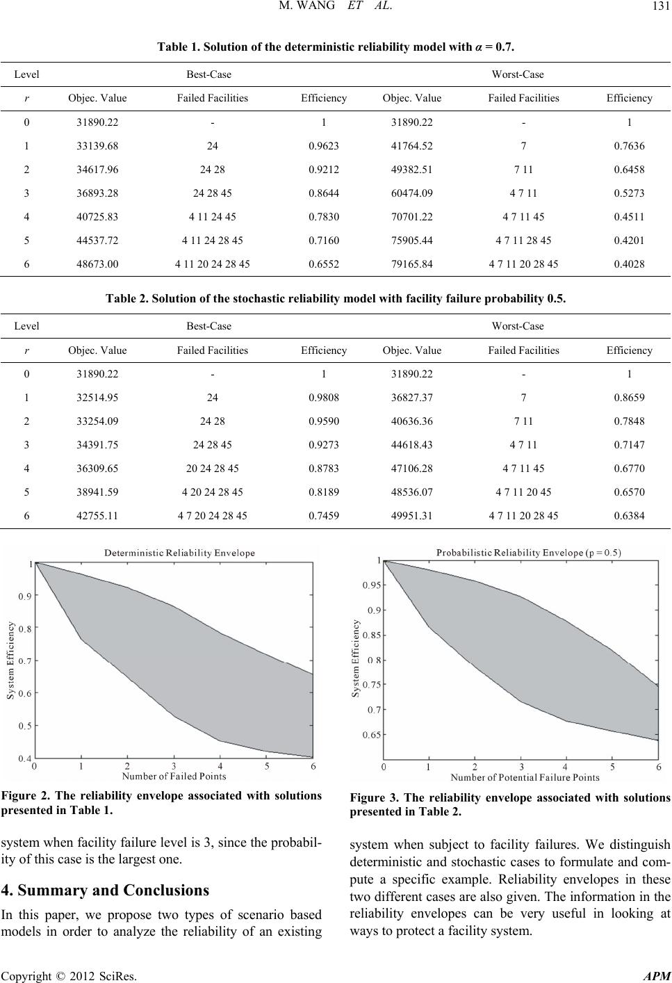

M. WANG ET AL.

APM

131

Table 1. Solution of the deterministic reliability model with α = 0.7.

Level Best-Case Worst-Case

r Objec. Value Failed Facilities Efficiency Objec. Value Failed Facilities Efficiency

0 31890.22 - 1 31890.22 - 1

1 33139.68 24 0.9623 41764.52 7 0.7636

2 34617.96 24 28 0.9212 49382.51 7 11 0.6458

3 36893.28 24 28 45 0.8644 60474.09 4 7 11 0.5273

4 40725.83 4 11 24 45 0.7830 70701.22 4 7 11 45 0.4511

5 44537.72 4 11 24 28 45 0.7160 75905.44 4 7 11 28 45 0.4201

6 48673.00 4 11 20 24 28 45 0.6552 79165.84 4 7 11 20 28 45 0.4028

Table 2. Solution of the stochastic reliability model with facility failure probability 0.5.

Level Best-Case Worst-Case

r Objec. Value Failed Facilities Efficiency Objec. Value Failed Facilities Efficiency

0 31890.22 - 1 31890.22 - 1

1 32514.95 24 0.9808 36827.37 7 0.8659

2 33254.09 24 28 0.9590 40636.36 7 11 0.7848

3 34391.75 24 28 45 0.9273 44618.43 4 7 11 0.7147

4 36309.65 20 24 28 45 0.8783 47106.28 4 7 11 45 0.6770

5 38941.59 4 20 24 28 45 0.8189 48536.07 4 7 11 20 45 0.6570

6 42755.11 4 7 20 24 28 45 0.7459 49951.31 4 7 11 20 28 45 0.6384

Figure 2. The reliability envelope associated with solutions

presented in Table 1. Figure 3. The reliability envelope associated with solutions

presented in Table 2.

system when facility failure level is 3, since the probabil-

ity of this case is the largest one. system when subject to facility failures. We distinguish

deterministic and stochastic cases to formulate and com-

pute a specific example. Reliability envelopes in these

two different cases are also given. The information in the

reliability envelopes can be very useful in looking at

ways to protect a facility system.

4. Summary and Conclusions

In this paper, we propose two types of scenario based

models in order to analyze the reliability of an existing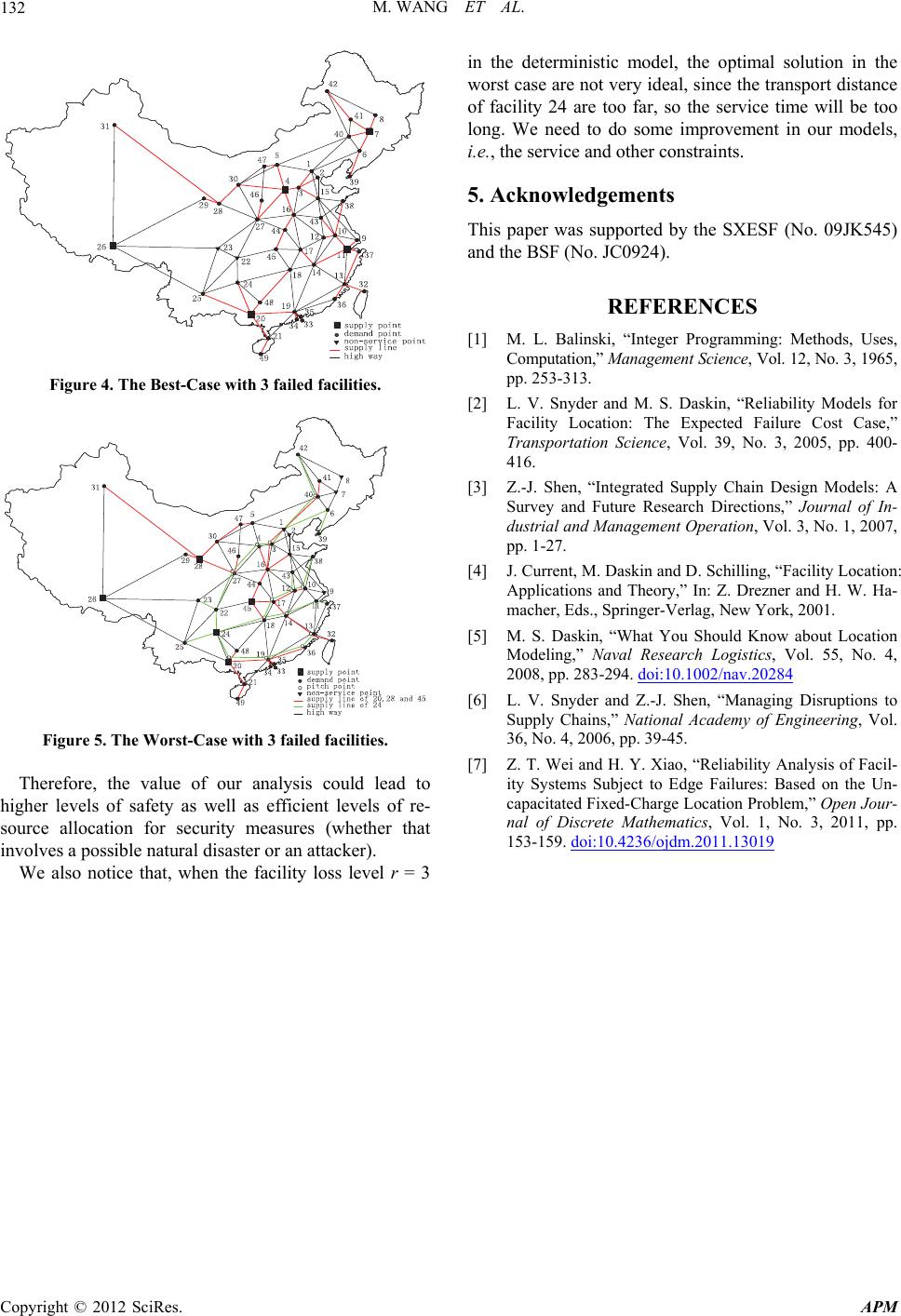

M. WANG ET AL.

132

Figure 4. The Best-Case with 3 fail e d facilities.

Figure 5. The Worst-Case with 3 failed facilities.

Therefore, the value of our analysis could lead to

higher levels of safety as well as efficient levels of re-

source allocation for security measures (whether that

involves a possible natural disaster or an attacker).

We also notice that, when the facility loss level r = 3

in the deterministic model, the optimal solution in the

worst case are not very ideal, since the transport distance

of facility 24 are too far, so the service time will be too

long. We need to do some improvement in our models,

i.e., the service and other constraints.

5. Acknowledgements

This paper was supported by the SXESF (No. 09JK545)

and the BSF (No. JC0924).

REFERENCES

[1] M. L. Balinski, “Integer Programming: Methods, Uses,

Computation,” Mana gement Science, Vol. 12, No. 3, 1965,

pp. 253-313.

[2] L. V. Snyder and M. S. Daskin, “Reliability Models for

Facility Location: The Expected Failure Cost Case,”

Transportation Science, Vol. 39, No. 3, 2005, pp. 400-

416.

[3] Z.-J. Shen, “Integrated Supply Chain Design Models: A

Survey and Future Research Directions,” Journal of In-

dustrial and Management Operation, Vol. 3, No. 1, 2007,

pp. 1-27.

[4] J. Current, M. Daskin and D. Schilling, “Facility Location:

Applications and Theory,” In: Z. Drezner and H. W. Ha-

macher, Eds., Springer-Verlag, New York, 2001.

[5] M. S. Daskin, “What You Should Know about Location

Modeling,” Naval Research Logistics, Vol. 55, No. 4,

2008, pp. 283-294. doi:10.1002/nav.20284

[6] L. V. Snyder and Z.-J. Shen, “Managing Disruptions to

Supply Chains,” National Academy of Engineering, Vol.

36, No. 4, 2006, pp. 39-45.

[7] Z. T. Wei and H. Y. Xiao, “Reliability Analysis of Facil-

ity Systems Subject to Edge Failures: Based on the Un-

capacitated Fixed-Charge Location Problem,” Open Jour-

nal of Discrete Mathematics, Vol. 1, No. 3, 2011, pp.

153-159. doi:10.4236/ojdm.2011.13019