A Semi Automated Method for Laminated Sediments Analysis

doi:10.4236/ijg.2012.31023

Paper Menu >>

Journal Menu >>

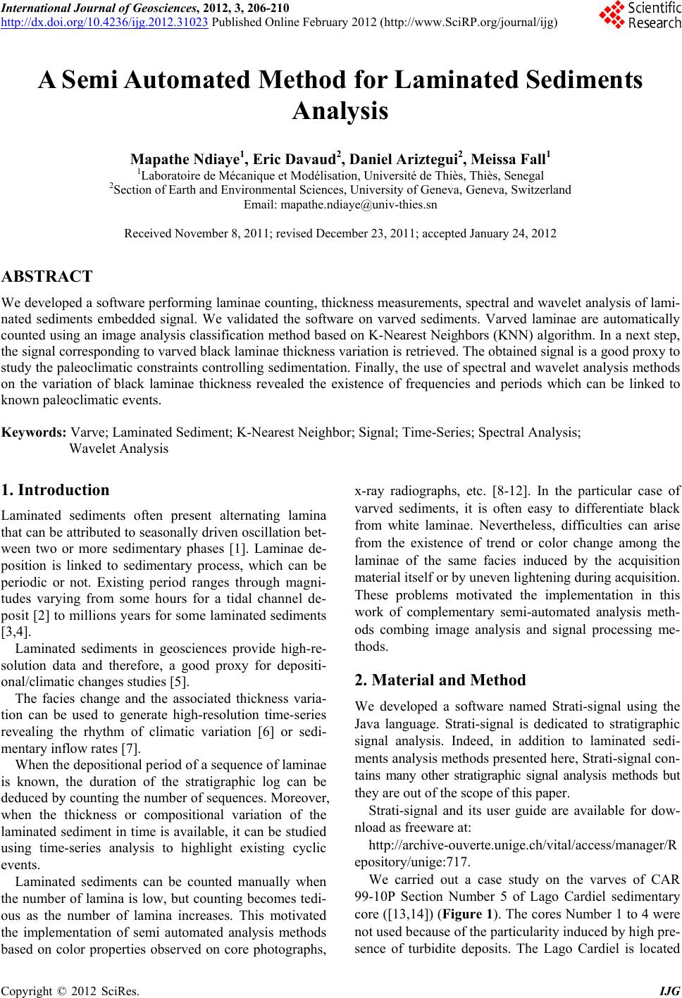International Journal of Geosciences, 2012, 3, 206-210

http://dx.doi.org/10.4236/ijg.2012.31023 Published Online February 2012 (http://www.SciRP.org/journal/ijg)

A Semi Automated Method for Laminated Sediments

Analysis

Mapathe Ndiaye1, Eric Davaud2, Daniel Ariztegui2, Meissa Fall1

1Laboratoire de Mécanique et Modélisation, Université de Thiès, Thiès, Senegal

2Section of Earth and Environmental Sciences, University of Geneva, Geneva, Switzerland

Email: [email protected]

Received November 8, 2011; revised December 23, 2011; accepted January 24, 2012

ABSTRACT

We developed a software performing laminae counting, thickness measurements, spectral and wavelet analysis of lami-

nated sediments embedded signal. We validated the software on varved sediments. Varved laminae are automatically

counted using an image analysis classification method based on K-Nearest Neighbors (KNN) algorithm. In a next step,

the signal corresponding to varv ed black laminae thickness variatio n is retrieved. The obtained sign al is a good proxy to

study the paleoclimatic constraints controlling sedimentation. Finally, the use of spectral and wavelet analysis methods

on the variation of black laminae thickness revealed the existence of frequencies and periods which can be linked to

known paleoclimatic events.

Keywords: Varve; Laminated Sediment; K-Nearest Neighbor; Signal; Time-Series; Spectral Analysis;

Wavelet Analysis

1. Introduction

Laminated sediments often present alternating lamina

that can be attribu ted to seasonally driven oscillation bet-

ween two or more sedimentary phases [1]. Laminae de-

position is linked to sedimentary process, which can be

periodic or not. Existing period ranges through magni-

tudes varying from some hours for a tidal channel de-

posit [2] to millions years for some laminated sediments

[3,4].

Laminated sediments in geosciences provide high-re-

solution data and therefore, a good proxy for depositi-

onal/climatic chang es studies [5].

The facies change and the associated thickness varia-

tion can be used to generate high-resolution time-series

revealing the rhythm of climatic variation [6] or sedi-

mentary inflow rates [7].

When the depositional period of a sequence of laminae

is known, the duration of the stratigraphic log can be

deduced by cou nting the numb er of sequences. Moreov er,

when the thickness or compositional variation of the

laminated sediment in time is availab le, it can be studied

using time-series analysis to highlight existing cyclic

events.

Laminated sediments can be counted manually when

the number of lamina is low, but counting becomes tedi-

ous as the number of lamina increases. This motivated

the implementation of semi automated analysis methods

based on color properties observed on core photographs,

x-ray radiographs, etc. [8-12]. In the particular case of

varved sediments, it is often easy to differentiate black

from white laminae. Nevertheless, difficulties can arise

from the existence of trend or color change among the

laminae of the same facies induced by the acquisition

material itself or by uneven lightening during acquisition.

These problems motivated the implementation in this

work of complementary semi-automated analysis meth-

ods combing image analysis and signal processing me-

thods.

2. Material and Method

We developed a software named Strati-signal using the

Java language. Strati-signal is dedicated to stratigraphic

signal analysis. Indeed, in addition to laminated sedi-

ments analysis methods presented here, Strati-signal con-

tains many other stratigraphic signal analysis methods but

they are out of the scope of this paper.

Strati-signal and its user guide are available for dow-

nload as freeware at:

http://archive-ouverte.unige.ch/vital/access/manager/R

epository/unige:717.

We carried out a case study on the varves of CAR

99-10P Section Number 5 of Lago Cardiel sedimentary

core ([13,14]) (Figure 1). The cores Number 1 to 4 were

not used because of the particularity induced by high pre-

sence of turbidite deposits. The Lago Cardiel is located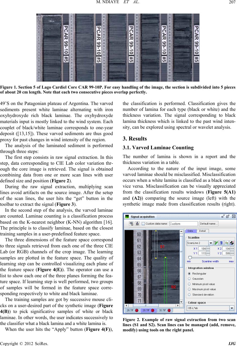

M. NDIAYE ET AL. 207

Figure 1. Section 5 of Lago Cardiel Core CAR 99-10P. For easy handling of the image, the section is subdivided into 5 pieces

of about 20 cm length. Note that each two consecutive pieces overlap perfectly.

49˚S on the Patagonian plateau of Argentina. The varved

sediments present white laminae alternating with iron

oxyhydroxyde rich black laminae. The oxyhydroxyde

materials input is mostly linked to the wind system. Each

couplet of black/white laminae corresponds to one-year

deposit ([13,15]). These varved sediments are thus good

proxy for past changes in wind intensity of the region.

The analysis of the laminated sediment is performed

through three steps:

The first step consists in raw signal extraction. In this

step, data corresponding to CIE Lab color variation thr-

ough the core image is retrieved. The signal is obtained

combining data from one or more scan lines with user

defined size and position (Figure 2).

During the raw signal extraction, multiplying scan

lines avoid artifacts on the source image. After the setup

of the scan lines, the user hits the “get” button in the

toolbar to extract the signal (Figure 3).

In the second step of the analysis, the varved laminae

are counted. Laminae counting is a classification process

based on the K-nearest neighbor (K-NN) algorithm [16].

The principle is to classify laminae, based on the closest

training samples in a user-predefined feature space.

The three dimensions of the feature space correspond

to three signals retrieved from each one of the three CIE

Lab (or RGB) channels of the crop image. The learning

samples are plotted in the feature space. The quality of

learning step can be controlled visualizing each plane of

the feature space (Figure 4(E)). The operator can use a

list to show each one of the three planes forming the fea-

ture space. If learning step is well performed, two groups

of samples will be formed in the feature space corre-

sponding respectively to white and black laminae.

The training samples are got by successive mouse cli-

cks on a user-desired part of the synthetic image (Figure

4(B)) to pick significative samples of white or black

la min a e . I n oth e r wo r d s, t h e user indicates su ccess ively to

the classifier what a black lamina and a white lamina is.

When the user hits the “Apply” button (Figure 4(F)),

the classification is performed. Classification gives the

number of lamina for each type (black or white) and the

thickness variation. The signal corresponding to black

lamina thickness which is linked to the past wind inten-

sity, can be explored using spectral or wavelet analysis.

3. Results

3.1. Varved Laminae Counting

The number of lamina is shown in a report and the

thickness variation in a tab le.

According to the nature of the input image, some

varved laminae should be misclassified. Misclassification

occurs when a white lamina is classified as a black one or

vice versa. Misclassification can be visually appreciated

from the classification results windows (Figure 5(A1)

and (A2)) comparing the source image (left) with the

synthetic image made from classification results (right).

Figure 2. Example of raw signal extraction from two scan

lines (S1 and S2). Scan lines can be managed (add, remove,

modify) using tools on the right panel.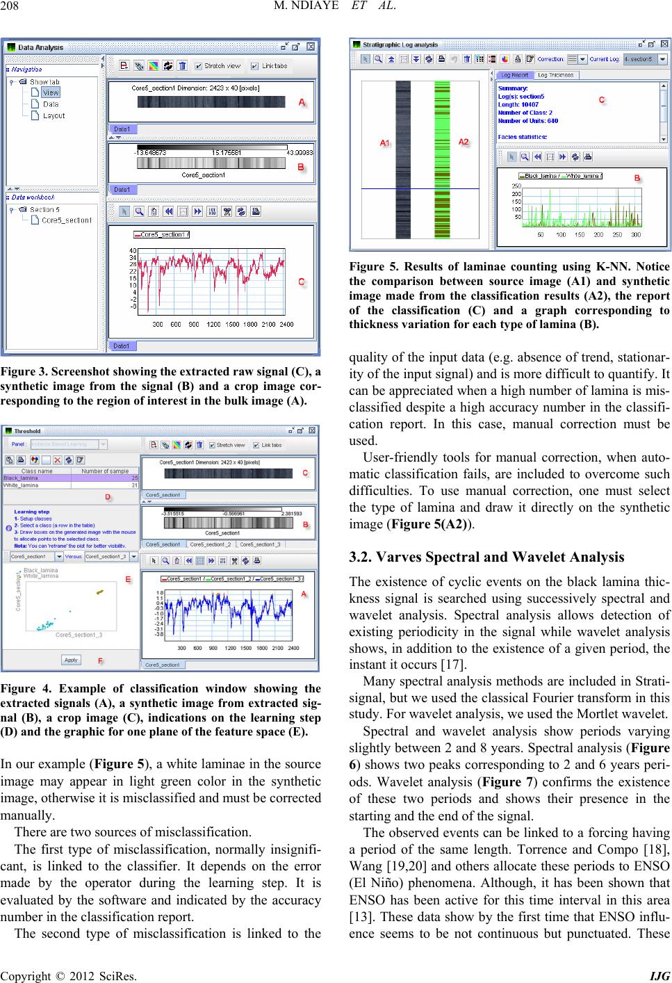

M. NDIAYE ET AL.

208

Figure 3. Screenshot showing the extracted raw signal (C), a

synthetic image from the signal (B) and a crop image cor-

responding to the region of interest in the bulk image (A).

Figure 4. Example of classification window showing the

our example (Figure 5), a white laminae in the source

e two sources of misclassification. insignifi-

tion is linked to the

extracted signals (A), a synthetic image from extracted sig-

nal (B), a crop image (C), indications on the learning step

(D) and the graphic for one plane of the feature space (E).

image may appear in light green color in the synthetic

image, otherwise it is misclassified and must be corrected

manually.

There ar

The first type of misclassification, normally

nt, is linked to the classifier. It depends on the error

made by the operator during the learning step. It is

evaluated by the software and indicated by the accuracy

number in the classification report.

The second type of misclassifica

Figure 5. Results of laminae counting using K-NN. Notice

uality of the input data (e.g. absence of tren d, stationar-

r-friendly tools for manual correction, when auto-

3.2. Varves Spectral and Wavelet Analysis

a thic-

sis methods are included in Strati-

the comparison between source image (A1) and synthetic

image made from the classification results (A2), the report

of the classification (C) and a graph corresponding to

thickness variation for each type of lamina (B).

ity of the input signal) and is more difficu lt to quantify. It

can be appreciated when a high number of lamina is mis-

classified despite a high accuracy number in the classifi-

cation report. In this case, manual correction must be

used.

Use

atic classification fails, are included to overcome such

difficulties. To use manual correction, one must select

the type of lamina and draw it directly on the synthetic

image (Figure 5(A2)).

The existence of cyclic events on the black lamin

kness signal is searched using successively spectral and

wavelet analysis. Spectral analysis allows detection of

existing periodicity in the signal while wavelet analysis

shows, in addition to the existence of a given period, the

instant it occurs [17 ].

Many spectral analy

gnal, but we used the classical Fou rier transform in this

study. For wavelet analysis, we used the Mortlet wavelet.

Spectral and wavelet analysis show periods varying

ightly between 2 and 8 years. Spectral analysis (Figure

6) shows two peaks corresponding to 2 and 6 years peri-

ods. Wavelet analysis (Figure 7) confirms the existence

of these two periods and shows their presence in the

starting and the end of the signal.

The observed events can be linked to a forcing having

period of the same length. Torrence and Compo [18],

Wang [19,20] and others allocate these periods to ENSO

(El Niño) phenomena. Although, it has been shown that

ENSO has been active for this time interval in this area

[13]. These data show by the first time that ENSO influ-

ence seems to be not continuous but punctuated. These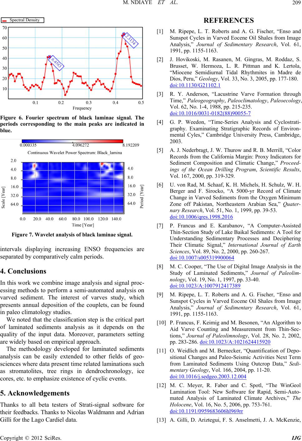

M. NDIAYE ET AL. 209

Figure 6. Fourier spectrum of black laminae signal. The

periods corresponding to the main peaks are indicated in

blue.

Figure 7. Wavelet analysis of black laminae signal.

tervals displaying increasing ENSO frequencies a

4. Conclusions

bine image analysis and signal proc

tion step is the critical part

ed sediments

5. Acknowledgements

f Strati-signal software fo

CES

[1] M. Ripepe, L. T. Roberts and A. G. Fischer, “Enso and

Sunspot CycleShales from Image

Analysis,” Jo esearch, Vol. 61,

l Tidal Rhythmites in Madre de

inre

separated by comparatively calm periods.

In this work we com-

essing methods to perform a semi-automated analysis on

varved sediment. The interest of varves study, which

presents annual deposition of the couplets, can be found

in paleo climatology studies.

We noted that the classifica

laminated sediments analysis as it depends on the

quality of the input data. Moreover, parameters setting

are widely based on empirical approach.

The methodology developed for laminat

alysis can be easily extended to other fields of geo-

sciences where data pr esent time related laminations such

as stromatolites, tree rings in dendrochronology, ice

cores, etc. to emphasize existence of cyclic events.

Thanks to all beta testers or

the ir feedbacks. Thanks to Nicolas Waldmann a nd A dr ian

Gilli for the Lago Cardiel da ta.

REFEREN

s in Varved Eocene Oil

urnal of Sedimentary R

1991, pp. 1155-1163.

[2] J. Hovikoski, M. Rasanen, M. Gingras, M. Roddaz, S.

Brusset, W. Hermoza, L. R. Pittman and K. Lertola,

“Miocene Semidiurna

Dios, Peru,” Geology, Vol. 33, No. 3, 2005, pp. 177-180.

doi:10.1130/G21102.1

[3] R. Y. Anderson, “Lacustrine Varve Formation through

Time,” Paleogeography, Paleoclimatology, Paleoecology

Vol. 62, No. 1-4, 1988, ,

pp. 215-235.

doi:10.1016/0031-0182(88)90055-7

[4] G. P. Weedon, “Time-Series Analysis and Cyclostrati-

graphy. Examinating Stratigraphic R

mental Cyles,” Cambridge Universityecords of Environ-

Press, Cambridge,

nt Composition and Climatic Change,” Proceed-

from the Oxygen Minimum

2003.

[5] A. J. Nederbragt, J. W. Thurow and R. B. Merrill, “Color

Records from the California Margin: Proxy Indicators for

Sedime

ings of the Ocean Drilling Program, Scientific Results,

Vol. 167, 2000, pp. 319-329.

[6] U. von Rad, M. Schaaf, K. H. Michels, H. Schulz, W. H.

Berger and F. Sirocko, “A 5000-yr Record of Climate

Change in Varved Sediments

Zone off Pakistan, Northeastern Arabian Sea,” Quater-

nary Research, Vol. 51, No. 1, 1999, pp. 39-53.

doi:10.1006/qres.1998.2016

[7] P. Francus and E. Karabanov, “A Computer-Assisted

Thin- Sect ion Study of Lake Baikal Sediments: A

Understanding Sedimentary Tool for

Processes and Deciphering

Their Climatic Signal,” International Journal of Earth

Sciences, Vol. 89, No. 2, 2000, pp. 260-267.

doi:10.1007/s005319900064

[8] M. C. Cooper, “The Use of Digital Image Analysis in the

Study of Laminated Sediments,” Journal o

nology, Vol. 19, No. 1, 1997, f Paleolim-

pp. 33-40.

doi:10.1023/A:1007912417389

[9] M. Ripepe, L. T. Roberts and A. G. Fischer, “Enso and

Sunspot Cycles in Varved Eocene Oil Sh

Analysis,” Journal of Sedimenales from Image

tary Research, Vol. 61,

olimnology, Vol. 28, No. 2, 2002,

1991, pp. 1155-1163.

[10] P. Francus, F. Keimig and M. Besonen, “An Algorithm to

Aid Varve Counting and Measurement from Thin-Sec-

tions,” Journal of Pale

pp. 283-286. doi:10.1023/A:1021624415920

[11] O. Weidlich and M. Bernecker, “Quantification of Depo-

sitional Changes and Paleo-Seismic Activities Next Term

from Laminated Sediments Using Outcrop Data,” Sedi-

mentary Geology, Vol. 166, 2004, pp. 11-20.

doi:10.1016/j.sedgeo.2003.12.004

[12] M. C. Meyer, R. Faber and C. Spotl, “The WinGeol

Lamination Tool: New Software for Rapid,

mated Analysis of Laminated ClSemi-Auto-

imate Archives,” The

Holocene, Vol. 16, No. 5, 2006, pp. 753-761.

doi:10.1191/0959683606hl969rr

[13] A. Gilli, D. Ariztegui, F. S. Anselmetti, J. A. McKenzie,

M. NDIAYE ET AL.

210

ern Westerlies in South

V. Markgraf, I. Hajdas and R. D. McCulloch, “Mid-Holo-

cene Strengthening of the South

Ame ri ca—Sedimentological E vidences from Lago Cardiel,

Argentina (49˚S),” Global and Planetary Change, Vol.

49, No. 1-2, 2005, pp. 75-93.

doi:10.1016/j.gloplacha.2005.05.004

[14] N. Waldmann, D. Ariztegui, M. Ndiaye, A. Gilli and F. S.

Anselmetti, “Evidence of Late

Variability in Southernmost Patagoni

Holocene Wind Int

a-Lago Cardiel, Ar-

uthern Hemisphere: A

ensity

gentina,” Abstracts of the Thirteenth Meeting of Swiss

Sedimentologists, Fribourg, 2005.

[15] A. Gilli, F. S. Anselmetti, D. Ariztegui, J. P. Bradbury, R.

Kelts Kerry, V. Markgraf and J. A. McKenzie, “Tracking

Abrupt Climate Change in the So

Seismic Stratigraphic Study of Lago Cardiel, Argentina

(49˚S),” Terra Nova, Vol. 13, No. 6, 2001, pp. 443-448.

doi:10.1046/j.1365-3121.2001.00377.x

[16] B. V. Dasarathy, “Nearest Neighbor Pattern Classification

Techniques,” IEEE Press, California, 1991.

[17] E. P. Verrecchia, “Multiresolution Analysis of Shell

Natural Cy-

Growth Increments to Detect Variations in

cles,” Image Analysis, Sediments and Paleoenvironments,

Vol. 7, 2005, pp. 273-293.

doi:10.1007/1-4020-2122-4_14

[18] C. Torrence and G. P. Co

Wavelet Analysis,” Bulletin of

mpo, “A Practical Guide to

the American Meteoro-

logical Society, Vol. 79, No. 1, 1998, pp. 61-78.

doi:10.1175/1520-0477(1998)079<0061:APGTWA>2.0.

CO;2

[19] B. Wang, “Interdecadal Changes in El Niño Onset in the

Last F

our Decades,” Journal of Climate, Vol. 8, No. 2,

1995, pp. 267-285.

doi:10.1175/1520-0442(1995)008<0267:ICIENO>2.0.CO

[20] Y. Wang, “Temporal Structure of the Southern Oscilla-

tion as Revealed by Waveform and Wavelet Analysis,”

Journal of Climate, Vol. 9, No. 7, 1996, pp. 1586-1598.

doi:10.1175/1520-0442(1996)009<1586:TSOTSO>2.0.C

O;2