Qualititative Analysis of Interface Behavior under First Phase Transition

doi:10.4236/jcpt.2012.21005

Paper Menu >>

Journal Menu >>

Journal of Crystallization Process and Technology, 2012, 2, 25-29

http://dx.doi.org/10.4236/jcpt.2012.21005 Published Online January 2012 (http://www.SciRP.org/journal/jcpt)

Qualititative Analysis of Interface Behavior under First

Phase Transition

Alex Guskov

Institute of Solid State Physics of RAS, Moscow, Russia.

Email: [email protected]

Received October 25th, 2011; revised November 28th, 2011; accepted December 5th, 2011

ABSTRACT

At present there is no explanation of the nature of interface instability upon first order phase transitions. The well-

known theory of concentration overcooling under directed crystallization of solutions and Mullins-Sekerka instability

cannot account for the diversified liquid component redistribution during solid state transition. In [1-3], within the fra-

mework of the nonequilibrium mass transfer problem, it has been shown that there are regimes of the interface insta-

bility, which differ from the known ones [4-6]. Moreover, the instability theory of works [1-3] demonstrates a complete

experimental agreement of the dependence of eutectic pattern period on interface velocity. However, it is difficult to

explain interface instability within the framework of a general setting of the mass-transfer problem. This paper is de-

voted to qualitative analysis of the phenomena that are responsible for interface instability. The phenomena are con-

nected by a single equation. Qualitative analysis revealed a variety of different conditions responsible for instability of

flat interface stationary movement upon phase transition. The type of instability depends on system parameters. It is

important that interface instability in the asymptotic case of quasi-equilibrium problem setting is qualitatively different

from interface instability in the case of nonequilibrium problem setting.

Keywords: Phase Transition; Interface; Stability; Oscillation; Solution

1. Introduction

The heat-and-mass transfer problem under directed crys-

tallization is usually described by quasi-equilibrium bounda-

ry conditions [6-8]. Quasi-equilibrium problem setting has

a number of advantages. This statement was used for cal-

culation of numerous technological processes [7,8] that

are successfully used in crystal growth, met-allurgy and ma-

terials science. Yet, the quasi-equilibrium problem has its

disadvantages that in certain cases can be of principle sig-

nificance. For instance, in the problem with quasi-equoli-

brium boundary condition interface velocity cannot be con-

nected to the growth mechanism since it does not take into

account the nonequilibrium solution layer in front of the

interface. In [1-3] nonequilibrium problem setting is used

for description of the stability of the stationary regime of

directed crystallization. It is shown that the interface can

be unstable which accounts for the dynamics of component

redistribution upon phase transition. In particular, the de-

pendence of eutectic pattern period on interface velocity

was obtained. However, works [1-3] cannot explain the

obtained instability if the simple physical outline of

analysis and give a clear-cut distinction between the in-

terface dynamics of quasi-equilibrium problem setting

and that noneeqilibrium setting. This paper is intended to

make up for this deficiency.

2. Interface Stability

It is well known that first order phase transition occurs at

interface temperature which is different from equilibrium

temperature of phase transition. In particular, under crys-

tallization the temperature of crystallized liquid should

be less than the equilibrium crystallization temperature.

The difference between equilibrium temperature of phase

transition and current interface temperature is called ki-

netic overcooling. In quasi-equilibrium boundary condi-

tions kinetic overcooling is assumed to be equal to zero.

The equilibrium phase diagram is calculated subject to

the equality of phase chemical potentials. The chemical po-

tential values correspond to an infinite volume of each phase.

It is known, however, that the adsorption component for-

med on the interface is due to equality of the interface

chemical potentials. On phase transition the adsorption layer

affects interlayer component redistribution. Interface adsorp-

tion is commonly neglected in quasi-equilibrium bound-

ary conditions. The behavior of the adsorption layer upon

flat interface movement was considered by Hall [9]. Ac-

cording to Halls theory, there is relaxation time between

the component concentration in the layer and that in the

Qualititative Analysis of Interface Behavior under First Phase Transition

solid phase. Therefore, the interface velocity should be com-

pared to the diffusion coefficient as well as the relaxation

velocity of the component in the adsorption layer. Hall

introduced an effective distribution ratio equal to the com-

ponent solid phase-liquid solution concentration ratio. The

following expression was obtained for calculation of an

effective distribution ratio



=exp

ads

eff ads

KK KKv



 





Here eff

is the effective distribution ratio, k0 the

equilibrium distribution ratio, ads

the equilibrium ad-

sorption distribution ratio, ads the constant velocity of

adsorption, V the crystallization velocity. Let us consider

the physical meaning of this formula. To maintain the

composition of the adsorption layer, it is required that the

velocity of diffusion of component atoms from the melt

to the crystal exceeds the interface velocity. Hence, the

dissolved component concentration gradient might occur,

for instance, in the opposite direction and, as a result, in

front of the crystal there appears a depleted region in-

stead of the accumulation one corresponding to the equi-

librium phase diagram without regard for interface ad-

sorption. In this case the values of the effective distribu-

tion ratio will get from the region where eff

< 1 with

the equilibrium distribution ratio 0

< 1 over to the

region eff

> 1. Within the limit of high interface ve-

locities the distribution ratio will approach the adsorption

distribution ratio eff

= ads

. Interface temperature and

equilibrium phase transition temperature are differently

dependent on temperature and concentration varies of sys-

tem. For instance, equilibrium phase transition tempera-

ture is essentially dependent on component concentration

in front of the interface. Therefore, in accordance with

the phase diagram, at eff

< 1, equilibrium phase transi-

tion temperature decreases (considering 0

< 1) with in-

creasing component concentration. This results in decreased

kinetic overcooling as well as decreased interface veloc-

ity. The latter leads to decreasing concentration which

returns to its initial value. The interface is stability. De-

crease of interface velocity at eff

> 1 leads to further

increase of concentration which accounts for interface in-

stability.

Write kinetic overcooling in the form:



ke e

TT mCCT



 

Here Te∞ is the phase transition equilibrium tempera-

ture of the initial solution, Ce∞ the concentration of the

initial solution, T0 and C0 the interface temperature and

concentration of the solution, respectively. The interface

velocity is a monotonically increasing function of kinetic

overcooling . We distinguish two cases of the

solution state in the overcooled layer in front of the in-

terface: the cases of stable and instable solution [3]. For

definiteness we will consider a eutectic phase diagram for

the case when liquid solution concentration is less than

eutectic concentration, 0



vvT



< 1, the liquidus slope being

negative, m < 0. Let the flat interface in the stationary

regime move at a velocity Vs. Therefore, at eff

< 1, m

< 0, the interface is stable. But it is well known that this

may lead to concentration instability associated with the

so-called concentration overcooling [4]. If the tempera-

ture gradient of the liquid solution on the interface is less

than the gradient of the phase transition equilibrium tem-

perature, the interface may lose its stability. In the non-

equilibrium case it can be explained as follows. Let inter-

face temperature T0 decrease due to fluctuations. This

will involve increased kinetic overcooling and, hence, in-

creased interface velocity. There appears an asperity in the

region of concentration overcooling, i.e. an increase in the

interface equilibrium temperature of phase transition. This

involves an increase in kinetic overcooling as well as fur-

ther increase of interface velocity. Hence, the presence of

a concentration overcooling region leads to interface in-

stability. On the other hand, consideration of kinetic insta-

bility yields that increased interface velocity involves an

increase in interface component concentration. This will

decrease equilibrium temperature of phase transition and,

therefore, decrease kinetic overcooling and interface ve-

locity. These two inverse processes can be illustrated by

the following scheme:

TTv

CTv



  



Thus, we have obtained inverse variations of equilib-

rium temperature of phase transition. On the one hand, it

increases due to local interface movement; on the other

hand, it decreases due to edging of the component by the

interface and change of kinetic overcooling. The two in-

verse processes can either lead to or fail to lead to inter-

face instability which depends on the external conditions

and the physical parameters of the system.

3. Equation of Interface Oscillations

Let us find the relationship between temperature and con-

centration perturbations and small interface movement

zm (t) from the interface coordinate z = 0 of stationary

regime. Linearize interface movement velocity by concen-

tration and temperature perturbations [1,3]

















000 0

kkS

vTTC TC

mC TV





 (1)

Here







. As shown above, we consider a qua-

litative model of interface movement dynamics. Heat con-

duction, diffusion and phase transition heat affecting spa-

Qualititative Analysis of Interface Behavior under First Phase Transition

tial distribution of temperature and concentration are ne-

glected. The aim is to show the feasible reasons behind in-

terface instability using the relationship between the lump-

ed interface parameters. The interface temperature varia-

tion at distance zm (t) in the linear approximation can be

written as

where



00 0

ddS

CC CV











 





)



mmS zmm

Tzt gradTzgradTzzt











Substitute the small temperature and concentration varia-

tions from (2) and (3) into (1). Upon elementary trans-

formations we obtain the equation

(2)

dd 0

ahgz



 (4)

In harmonic analysis of interface stability the function

Tm (z) was found as the solution of a common differential

equation [2] and depended on time frequency and wave

number. Here we do not consider spatial distribution of

temperature and concentration; rather follow small time

variations of the interface temperature and concentration.

Thus, in (2) the spatial gradient of small temperature per-

turbation is neglected. To connect concentration perturba-

tion with interface movement, let us use the known rela-

tion between pulse variation of interface velocity and in-

terface variation of concentration upon stationary move-

ment of the interface [4]. If the distribution ratio is <1,

the velocity increase leads to increase of concentration

which then returns to its original value. If the distribution

ratio is >1, the velocity increase first leads to decrease of

concentration which then returns to its stationary value.

Thus, interface concentration is dependent on velocity va-

riation. Consider also variation of concentration at the mo-

vement of the interface zm (t) owing to the spatial varia-

tion of the concentration of the stationary regime. For the

same conditions as in the case of (2) the linear approxi-

mation for concentration variation yields

where



gradCzgrad Tz

 1





The parameters α and g are dependent on stationary

interface velocity. The parameter h > 0 is independent of

the movement interface regime. It involves only parame-

ters dependent on the nature of the solution. The stability

and form of the nonsimple point



t = 0 depend on

the relationship between the coefficients of Equation (4).

This is the well-known linear oscillator equation and its

solutions are thoroughly studied in [10].

4. Nonsimple Point Type of System

 



00 0

d()

CtCagrad Cs zzTCC

t

 

0Sm

To describe stability of stationary interface movement upon

perturbations of temperature and concentration, let us di-

vide the regimes into groups by the characteristics shown

in Table 1. The sign of α indicates whether the compo-

nent is edged or captured by the solid phase. The sign of

the stationary concentration distribution gradient gradCS

together with α indicates whether the nonequilibrium so-

lution layer in front of the interface is in the stable or me-

tastable state. The discriminant sign of the characteristic

equation indicates whether at given parameters Equation

(3)

Table 1. The nonsimple point zm (t) = 0 type at the vary values of the Equation (4) parameters.

α gradCS h g det zm = 0

Equilibrium α > 0 gradCS = 0 h > 0 g = 0 det = h2 − g = h2 stable exponent

gradTS ≠ 0 α > 0 gradCS = 0 h > 0 g > 0 det > 0 stable node

gradTS ≠ 0 α > 0 gradCS = 0 h > 0 g > 0 det > 0 stable focus

1 α > 0 gradCS < 0 h > 0 g > 0 det > 0 stable node

2 α > 0 gradCS < 0 h > 0 g > 0 det < 0 stable focus

3 α > 0 gradCS > 0 h > 0 g > 0 det > 0 stable node

4 α > 0 gradCS > 0 h > 0 g > 0 det > 0 stable focus

5 α > 0 gradCS < 0 h > 0 g < 0 det > 0 saddle

6 α < 0 gradCS > 0 h < 0 g < 0 det > 0 saddle

7 α < 0 gradCS < 0 h < 0 g < 0 det > 0 saddle

8 α < 0 gradCS < 0 h < 0 g > 0 det < 0 nonstable node

9 α < 0 gradCS < 0 h < 0 g > 0 det < 0 nonstable focus

Qualititative Analysis of Interface Behavior under First Phase Transition

(4) has real or complex characteristic numbers. Let us give

a brief description of the regimes presented.

In the equilibrium state g = 0, α > 0 (k = k0). Equation

(4) gives stable solutions. In the equilibrium regime any

perturbation involves finite movement of the interface. The

system asymptotically approaches the equilibrium state

at large values of t. Two regimes with gradTS ≠ 0 and a

motionless interface represent the initial state of the sys-

tem. These regimes are introduced to emphasize that even

with a motionless interface the system is in the nonequi-

librium state. If in the equilibrium state the coordinate

point (a, g) is on the a axis, then at VS = 0 the coordinate

point can be anywhere within the interval (a > 0, g > 0).

Depending on the sign of det, the point of the parameter

values can be either a stable node or a stable focus. Re-

gimes 1 and 2 exhibit a qualitatively identical temperature

and concentration distribution. The nonsimple point is sta-

ble. The sign of det determines whether it will be a node

or a focus. It should be noted that with changing velocity

the nonsimple point can have either node-focus or focus-

node bifurcation. Phase portrait on Figure 1 shows regions

with different types of nonsimple points. The figures in

the circles indicate the range of system parameter values

corresponding to the row number in Table 1. Regimes 3

and 4 are different from 1 and 2 only by the sign of the

concentration gradient. This corresponds to solution insta-

bility in the kinetic overcooling region .The change of the

concentration sign gradient leads to the fact that g > 0 at

any stationary interface velocity. Regime 5 is the bifurca-

tion of the nonsimple point of Regimes 1 and 2 when g be-

comes negative. This sign reversal indicates transition to

the concentration overcooling region. It should be empha-

sized that this regime requires a well-developed concen-

tration profile and, hence, a fairly high interface velocity.

Regimes 6 - 9 are different from 1 - 5 regimes by the sign

of parameter a. These regimes can be implemented pro-

vided the interface velocity of the stationary regime is suf-

ficiently large for the distribution ratio to exceed unity due

to interface component adsorption. Regimes 1 and 2 can

change to Regime 6 which is actually transition of stable

solution from a regime with a > 0 to that with a < 0 at an

Figure 1. Phase portrait of nonequilibrium system.

interface velocity sufficient for interface component ad-

sorption. By transition between stable regimes with dif-

ferent values of stationary interface velocity we mean a slow

change of stationary interface velocity without failure of

the flat interface surface. As the stable regime changes to an

instable one, the interface in experiments can remain flat

only to the stability boundary. Further interface dynamics is

determined by the domain of attraction of some steady-state

regime of the system. Transient and steady-state regimes

cannot be considered in this qualitative analysis. As it

follows from the analysis, depending on parameter gradCS

and a with increasing velocity of the stationary regime,

stable solutions 1 and 2 can formally change into one of

the two instable solutions: Regime 5 related to transition

of the stable regime to the concentration over-cooling re-

gime or Regime 6 related to transition of the distribution

ratio to the region with eff

> 1 owing to interface com-

ponent adsorption. Regimes 3 and 4 can change to re-

gime 7 since they all have instable solution in front of the

interface. Regimes 3 and 4 can also change to Regime 8

and 9 provided the sign of parameter α is changed, i.e.

due to adsorption, the effective distribution ration be-

comes greater than unity and changes the sign of g and the

system gets over to the concentration overcooling region.

Now let us consider quasiequilibrium problem setting.

In the equation obtained the kinetic coefficient 1/Λ stands

for a dissipative term. The smaller 1/Λ, the larger Λ and,

hence, the higher the interface velocity at the same kine-

tic overcooling. In the limit Λ = ∞ (h = 0) at any infinite-

simal kinetic overcooling the interface immediately shifts

to the equilibrium phase transition surface. In this case ki-

netic overcooling tends to zero whereas the equilibrium

temperature tends to equilibrium phase transition tempe-

rature, i.e. the regime corresponds to quasiequilibrium set-

ting of the directed crystallization problem. Within the li-

mit Λ = ∞ Equation (4) transforms to a harmonic oscilla-

tor equation which yields two variants of solution, namely,

solutions with imaginary characteristic numbers α > 0, g

> 0 or, which is formally the same, α < 0, g < 0. Here the

nonsimple point is the center, And solutions with real

characteristic equal sign numbers α > 0, g < 0 or, which

is formally the same, α < 0, g > 0, the nonsimple point

being a saddle. Figure 2 shows a phase portrait of non-

simple points for Equation (4) at h = 0. In the general case

the phase portrait of the system should be considered in

the three- dimensional system (α, g, h). If the coefficient

h of the oscillation equation is taken as a control pa-

rameter, the value of h = 0 is presented as a special case

of fixed physical parameters of the system and the phase

portrait of nonsimple points shown in Figure 2 belongs

to the case of a noncoarse dynamic system. The value h =

0 corresponds to the zero value of kinetic overcooling.

Strictly speaking, in this case the interface velocity is equal

to zero which does not imply equilibrium. The condition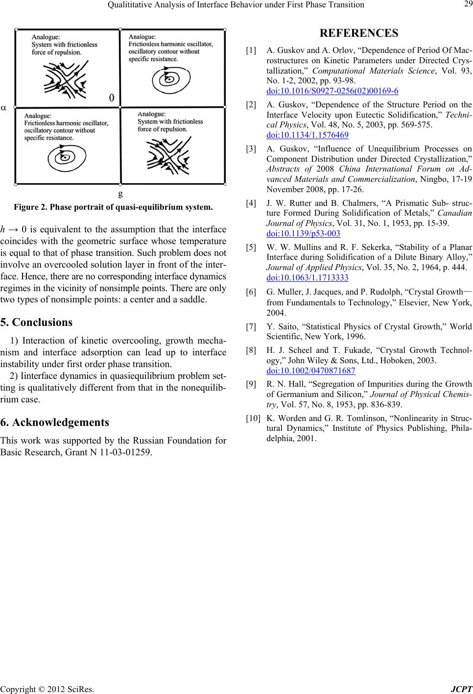

Qualititative Analysis of Interface Behavior under First Phase Transition 29

Figure 2. Phase portrait of quasi-equilibrium system.

h → 0 is equivalent to the assumption that the interface

coincides with the geometric surface whose temperature

is equal to that of phase transition. Such problem does not

involve an overcooled solution layer in front of the inter-

face. Hence, there are no corresponding interface dynamics

regimes in the vicinity of nonsimple points. There are only

two types of nonsimple points: a center and a saddle.

5. Conclusions

1) Interaction of kinetic overcooling, growth mecha-

nism and interface adsorption can lead up to interface

instability under first order phase transition.

2) Iinterface dynamics in quasiequilibrium problem set-

ting is qualitatively different from that in the nonequilib-

rium case.

6. Acknowledgements

This work was supported by the Russian Foundation for

Basic Research, Grant N 11-03-01259.

REFERENCES

[1] A. Guskov and A. Orlov, “Dependence of Period Of Mac-

rostructures on Kinetic Parameters under Directed Crys-

tallization,” Computational Materials Science, Vol. 93,

No. 1-2, 2002, pp. 93-98.

doi:10.1016/S0927-0256(02)00169-6

[2] A. Guskov, “Dependence of the Structure Period on the

Interface Velocity upon Eutectic Solidification,” Techni-

cal Physics, Vol. 48, No. 5, 2003, pp. 569-575.

doi:10.1134/1.1576469

[3] A. Guskov, “Influence of Unequilibrium Processes on

Component Distribution under Directed Crystallization,”

Abstracts of 2008 China International Forum on Ad-

vanced Materials and Commercialization, Ningbo, 17-19

November 2008, pp. 17-26.

[4] J. W. Rutter and B. Chalmers, “A Prismatic Sub- struc-

ture Formed During Solidification of Metals,” Canadian

Journal of Physics, Vol. 31, No. 1, 1953, pp. 15-39.

doi:10.1139/p53-003

[5] W. W. Mullins and R. F. Sekerka, “Stability of a Planar

Interface during Solidification of a Dilute Binary Alloy,”

Journal of Applied Physics, Vol. 35, No. 2, 1964, p. 444.

doi:10.1063/1.1713333

[6] G. Muller, J. Jacques, and P. Rudolph, “Crystal Growth—

from Fundamentals to Technology,” Elsevier, New York,

2004.

[7] Y. Saito, “Statistical Physics of Crystal Growth,” World

Scientific, New York, 1996.

[8] H. J. Scheel and T. Fukade, “Crystal Growth Technol-

ogy,” John Wiley & Sons, Ltd., Hoboken, 2003.

doi:10.1002/0470871687

[9] R. N. Hall, “Segregation of Impurities during the Growth

of Germanium and Silicon,” Journal of Physical Chemis-

try, Vol. 57, No. 8, 1953, pp. 836-839.

[10] K. Worden and G. R. Tomlinson, “Nonlinearity in Struc-

tural Dynamics,” Institute of Physics Publishing, Phila-

delphia, 2001.