Biclustering of time-lagged gene expression data using real number

doi:10.4236/jbise.2010.32029

Paper Menu >>

Journal Menu >>

J. Biomedical Science and Engineering, 2010, 3, 217-220

doi:10.4236/jbise.2010.32029 Published Online February 2010 (http://www.SciRP.org/journal/jbise/

JBiSE

Published Online February 2010 in SciRes. http://www.scirp.org/journal/jbise

Biclustering of time-lagged gene expression data using real

number

Feng Liu, Lingbing Wang

International School of Software, Wuhan University, China.

Email: [email protected]

Received 28 September 2008; revised 30 November 2009; accepted 30 December 2009.

ABSTRACT

Analysis of gene expression data can help to find the

time-lagged co-regulation of gene cluster. However,

existing method just solve the problem under the

condition when the data is discrete number. In this

paper, we propose efficient algorithm to indentify

time-lagged co-regulated gene cluster based on real

number.

Keywords: Microarray; Gene Expression; Bicluster;

Mean Squared Reside

1. INTRODUCTION

With the development of technology, some computa-

tional methods are widely used in the field of analyzing

gene expression data. Among them, the clustering and

biclustering techniques can detect the similar genes and

similar samples from the microarray based on the fact

that the similar genes have the similar expression levels

under the similar condition, which means that the sam-

ples should be gotten under the similar conditions such

as the sampling spot, sampling time and the sampling

temperatures. However, the samples are always gotten at

different period of time because the expression data are

always measured from different laboratory and different

purpose [1,2,3]. That is to say, the expression data re not

simultaneously co-expressing but time-lagged express-

ing. As a result, the genes expression products may af-

fect other genes’ expression during the biology process.

Such effect can be divided into two phenomenons: acti-

vation and inhibition. Under the activation process, one

gene expression can activate another gene expression.

On the contrary, a part of gene can inhibit the other gene

expression under the inhibition process. To be concluded,

some genes can activate or inhibit the other genes with

time lagged. That is defined as the time-lagged gene

expression. In this paper, we present an efficient method

to bicluster of the time-lagged gene expression data. In

the Section 2, we describe the related work. The method

is presented in Section 3. The experiment result is given

in Section 4 and the conclusion is given in Section 5.

2. RELATED WORKS

However, all the methods discussed above usually ana-

lyze two genes at the same time which have the draw-

backs as following: firstly, the approaches are clearly

computationally inefficient in practice. When given n

genes, n(n-1) times comparison cannot be avoided. Sec-

ondly, relationship between the genes is unclosed

enough using the methods. At the end, the methods

merely reflect the relationship between two genes rather

than various relationships among genes.

To solve the problems, Ji L. et al [3] presented an al-

gorithm to identify time-lagged gene clusters using gene

expression data. However, they just dealt with the dis-

crete data rather than the real data. In this paper, we

propose an algorithm to identify the localized time-lagg-

ed gene clusters from real data.

3. DEFINATIONS AND CONCEPTS

Definition 1. (Time-lagged Continuous Column Linear

Bicluster): Let G be the set of genes and T the set of

conditions (time spots). Let X(G,T) be the DNA expres-

sional matrix using real numbers. Let B(I, S, q) be the

subset of the expression data which denotes the ith gene’s

q continuous expression data from the time Si, where I is

the subset of G, S is a set of the ith gene’s expression

time, and q is the expression length. Then, B (I, S, q) is

defined as Time-lagged Continuous Column Linear Bi-

cluster only if each element is identical in difference ve-

ctors between rows (or columns) in the matrix B(I, S, q).

According to the definition mentioned above, there is

linear relationship between difference vectors in Time-

lagged Continuous Column Linear Bicluster B(I,S,q),

which are defined as the bicluster’s eigenvector.

Definition 2. (The Largest Time-lagged Continuous

Column Linear Bicluster): Let X(G,T) be the expression

matrix and B(I, S, q) the time-lagged continuous column

linear bicluster. If there isn’t any time-lagged continuous

column linear bicluster B’(I’, S’, q) which satisfies II’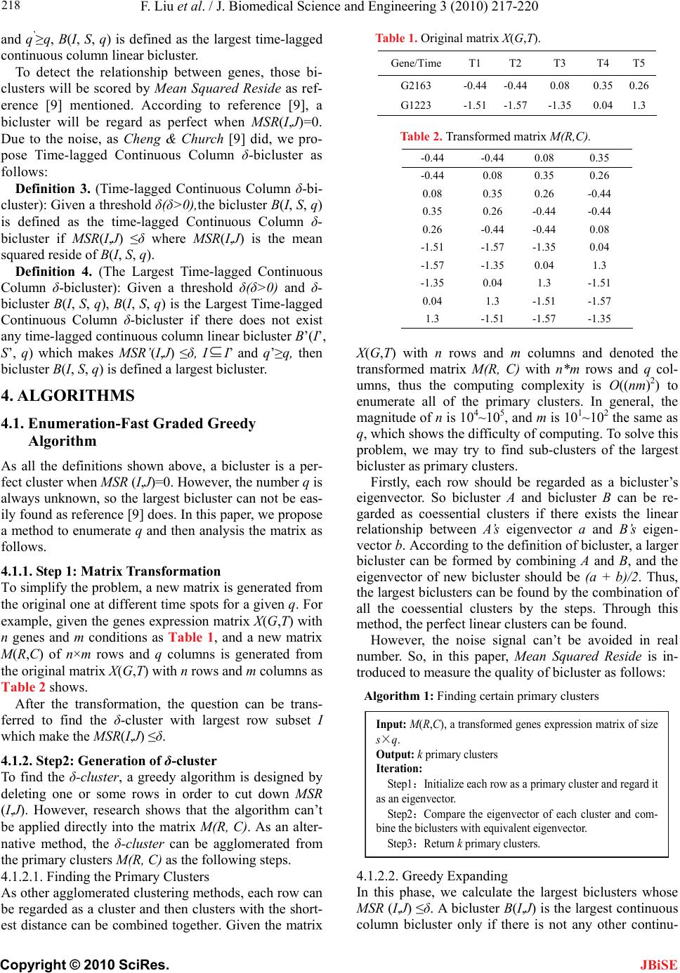

F. Liu et al. / J. Biomedical Science and Engineering 3 (2010) 217-220

218

JBiSE

and q’≥q, B(I, S, q) is defined as the largest time-lagged

continuous column linear bicluster.

To detect the relationship between genes, those bi-

clusters will be scored by Mean Squared Reside as ref-

erence [9] mentioned. According to reference [9], a

bicluster will be regard as perfect when MSR(I,J)=0.

Due to the noise, as Cheng & Church [9] did, we pro-

pose Time-lagged Continuous Column δ-bicluster as

follows:

Definition 3. (Time-lagged Continuous Column δ-bi-

cluster): Given a threshold δ(δ>0),the bicluster B(I, S, q)

is defined as the time-lagged Continuous Column δ-

bicluster if MSR(I,J) ≤δ where MSR(I,J) is the mean

squared reside of B(I, S, q).

Definition 4. (The Largest Time-lagged Continuous

Column δ-bicluster): Given a threshold δ(δ>0) and δ-

bicluster B(I, S, q), B(I, S, q) is the Largest Time-lagged

Continuous Column δ-bicluster if there does not exist

any time-lagged continuous column linear bicluster B’(I’,

S’, q) which makes MSR’ (I,J) ≤δ, II’ and q’≥q, then

bicluster B(I, S, q) is defined a largest bicluster.



4. ALGORITHMS

4.1. Enumeration-Fast Graded Greedy

Algorithm

As all the definitions shown above, a bicluster is a per-

fect cluster when MSR (I,J)=0. However, the number q is

always unknown, so the largest bicluster can not be eas-

ily found as reference [9] does. In this paper, we propose

a method to enumerate q and then analysis the matrix as

follows.

4.1.1. Step 1: Matrix Transformation

To simplify the problem, a new matrix is generated from

the original one at different time spots for a given q. For

example, given the genes expression matrix X(G,T) with

n genes and m conditions as Table 1, and a new matrix

M(R,C) of n×m rows and q columns is generated from

the original matrix X(G,T) with n rows and m columns as

Table 2 shows.

After the transformation, the question can be trans-

ferred to find the δ-cluster with largest row subset I

which make the MSR(I,J) ≤δ.

4.1.2. Step2: Generation of δ-cluster

To find the δ-cluster, a greedy algorithm is designed by

deleting one or some rows in order to cut down MSR

(I,J). However, research shows that the algorithm can’t

be applied directly into the matrix M(R, C). As an alter-

native method, the δ-cluster can be agglomerated from

the primary clusters M(R, C) as the following steps.

4.1.2.1. Finding the Primary Clusters

As other agglomerated clustering methods, each row can

be regarded as a cluster and then clusters with the short-

est distance can be combined together. Given the matrix

Table 1. Original matrix X(G,T).

Gene/Time T1 T2 T3 T4 T5

G2163 -0.44-0.44 0.08 0.350.26

G1223 -1.51-1.57 -1.35 0.041.3

Table 2. Transformed matrix M(R,C).

-0.44 -0.44 0.08 0.35

-0.44 0.08 0.35 0.26

0.08 0.35 0.26 -0.44

0.35 0.26 -0.44 -0.44

0.26 -0.44 -0.44 0.08

-1.51 -1.57 -1.35 0.04

-1.57 -1.35 0.04 1.3

-1.35 0.04 1.3 -1.51

0.04 1.3 -1.51 -1.57

1.3 -1.51 -1.57 -1.35

X(G,T) with n rows and m columns and denoted the

transformed matrix M(R, C) with n*m rows and q col-

umns, thus the computing complexity is O((nm)2) to

enumerate all of the primary clusters. In general, the

magnitude of n is 104~105, and m is 101~102 the same as

q, which shows the difficulty of computing. To solve this

problem, we may try to find sub-clusters of the largest

bicluster as primary clusters.

Firstly, each row should be regarded as a bicluster’s

eigenvector. So bicluster A and bicluster B can be re-

garded as coessential clusters if there exists the linear

relationship between A’s eigenvector a and B’s eigen-

vector b. According to the definition of bicluster, a larger

bicluster can be formed by combining A and B, and the

eigenvector of new bicluster should be (a + b)/2. Thus,

the largest biclusters can be found by the combination of

all the coessential clusters by the steps. Through this

method, the perfect linear clusters can be found.

However, the noise signal can’t be avoided in real

number. So, in this paper, Mean Squared Reside is in-

troduced to measure the quality of bicluster as follows:

Algorithm 1: Finding certain primary clusters

Input: M(R,C), a transformed genes expression matrix of size

s×q.

Output: k primary clusters

Iteration:

Step1：Initialize each row as a primary cluster and regard it

as an eigenvector.

Step2：Compare the eigenvector of each cluster and com-

bine the biclusters with equivalent eigenvector.

Step3：Return k primary clusters.

4.1.2.2. Greedy Expanding

In this phase, we calculate the largest biclusters whose

MSR (I,J) ≤δ. A bicluster B(I,J) is the largest continuous

column bicluster only if there is not any other continu-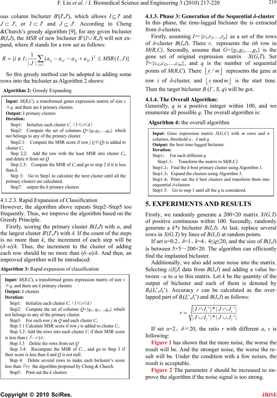

F. Liu et al. / J. Biomedical Science and Engineering 3 (2010) 217-220

219

JBiSE

ous column bicluster B'(I',J'), which allows II' and

J J', or I I' and J J'. According to Cheng

&Church’s greedy algorithm [9], for any given bicluster

B(I,J), the MSR of new bicluster B’(I∪R,J) will not ex-

pand, where R stands for a row set as follows:

 

}),()(

;{ 2







IJIjiJij JIMSRaaaa

IiR

So this greedy method can be adopted in adding some

rows into the bicluster as Algorithm 2 shows:

Algorithm 2: Greedy Expanding

Input: M(R,C), a transformed genes expression matrix of size s

×q, and there are k primary clusters

Output: k primary clusters

Iteration:

Step1: Initialize each cluster C

（1≤i≤k）

Step2: Compute the set of columns Q={q

,…,q

} which

not belongs to any of the primary cluster.

Step2.1: Compute the MSR score if row j (j∈Q) is added to

cluster C

Step 2.2: Add the row with the least MSR into cluster C

and delete it from set Q

Step 2.3: Compute the MSR of C

and go to step 2 if it is less

than δ.

Step 3: Go to Step1 to calculate the next cluster until all the

primary clusters are calculated.

Step7: output the k primary clusters

4.1.2.3. Rapid Expansion of Classification

However, the algorithm above repeats Step2~Step5 too

frequently. Thus, we improve the algorithm based on the

Greedy Principle.

Firstly, scoring the primary cluster B(I,J) with α, and

the largest cluster B'(I',J') with δ. If the count of the steps

is no more than k, the increment of each step will be

(δ–α)/k. Thus, the increment to the cluster of adding

each row should be no more than (δ–α)/k. And then, an

improved algorithm will be introduced:

Algorithm 3: Rapid expansion of classification

Input: M(R,C), a transformed genes expression matrix of size s

×q, and there are k primary clusters

Output: k clusters

Iteration:

Step1: Initialize each cluster C

（1≤i≤k）

Step2: Compute the set of columns Q={q

, q

,…,q

} which

not belongs to any of the primary cluster.

Step3: For each row j in Q and each cluster C

Step 3.1 Calculate MSR score if row j is added to cluster C

Step 3.2: Add the rows into each cluster C

if their MSR score

is less than (

)/r.

Step 3.3 Delete the rows from set Q

Step 3.4: Recompute the MSR of C

, and go to Step 3 if

their score is less than δ and Q is not null.

Step 4: Delete several rows to make each bicluster’s score

less than

by the algorithm proposed by Cheng & Church.

Step5: Print out the k clusters

4.1.3. Phase 3: Generation of the Sequential δ-cluster

In this phase, the time-lagged bicluster the is extracted

from δ-clusters.

Firstly, assuming I＝{r1,r2,…,rp} as a set of the rows

of δ-cluster B(I,J). There ri represents the ith row in

M(R,C). Secondly, assume that G={g1,g2,…,gn} is the

gene set of original expression matrix X(G,T). Set

T={ct1,ct2,…,ctm}, and q is the number of sequential

points of M(R,C). There /









mod

represents the gene at

row i of δ-cluster, and m







 is the start time.

Then the target bicluster B (I’, S, q) will be got.

4.1.4. The Overall Algorithm:

Generally, q is a positive integer within 100, and we

enumerate all possible q. The overall algorithm is:

Algorithm 4: the overall algorithm

Input: Gene expression matrix X(G,C) with m rows and n

columns, threshold α、δ and q.

Output: the best time-lagged bicluster.

Iteration:

Ste p1 ： For each different q

Ste p1 . 1： Transform the matrix to M(R,C)

Ste p1 . 2：Find the k-best primary cluster using Algorithm 1.

Ste p1 . 3：Expand the clusters using Algorithm 3.

Ste p1 . 4：Print out the k best clusters and transform them into

sequential δ-clusters

Step1.5: Go to step 1 until all the q is considered.

5. EXPERIMENTS AND RESULTS

Firstly, we randomly generate a 200×20 matrix X(G,T)

of positive continuous within 100. Secondly, randomly

generate a k*s bicluster B(I,J). At last, replace several

rows in X(G,T) by lines of B(I,J) at random points.

If set α=0.2、δ=1、k=4 、4≤q≤20, and the size of B(I,J)

is between 5×5～200×20. The algorithm can efficiently

find the implanted bicluster.

Additionally, we also add some noise into the matrix.

Selecting ε|I||J| data from B(I,J) and adding a value be-

tween –a to a to this matrix. Let k be the quantity of the

output of bicluster and each of them is denoted by

Bk(Ik’,Jk’). Accuracy r can be calculated as the over-

lapped part of Bi(Ii’,Ji’) and B(I,J) as follows:

|'|*|

IJJ





If set α=2、δ＝20, the ratio r with different a, ε is

following:

Figure 1 has shown that the more noise, the worse the

result will be. And the stronger noise, the worse the re-

sult will be. Under the condition with a few noises, the

result is acceptable.

Figure 2 The parameter δ should be increased to im-

prove the algorithm if the noise signal is too strong.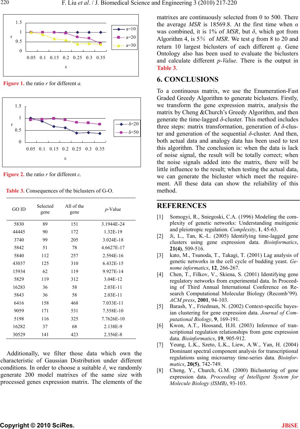

F. Liu et al. / J. Biomedical Science and Engineering 3 (2010) 217-220

220

0.5

1.5

0.05 0.1 0.15 0.2 0.25 0.3 0.35

a=10

a=20

a=30

JBiSE

Figure 1. the ratio r for different a.

0.5

1.5

0.050.10.150.20.250.30.35

δ=2 0

δ=5 0

Figure 2. the ratio r for different ε.

Table 3. Consequences of the biclusters of G-O.

GO ID Selected

gene

All of the

gene p-Value

5830 89 151 3.1944E-24

44445 90 172 1.32E-19

3740 99 205 3.024E-18

5842 51 78 4.6627E-17

5840 112 257 2.594E-16

43037 125 310 6.432E-15

15934 62 119 9.927E-14

5829 119 312 3.04E-12

16283 36 58 2.03E-11

5843 36 58 2.03E-11

6416 158 468 7.033E-11

9059 171 531 7.558E-10

5198 116 325 7.7626E-10

16282 37 68 2.138E-9

30529 141 423 2.356E-8

Additionally, we filter those data which own the

characteristic of Gaussian Distribution under different

conditions. In order to choose a suitable δ, we randomly

generate 200 model matrixes of the same size with

processed genes expression matrix. The elements of the

matrixes are continuously selected from 0 to 500. There

the average MSR is 18569.8. At the first time when α

was combined, it is 1% of MSR, but δ, which got from

Algorithm 4, is 5％ of MS R. We test q from 8 to 20 and

return 10 largest biclusters of each different q. Gene

Ontology also has been used to evaluate the biclusters

and calculate different p-Value. There is the output in

Table 3.

6. CONCLUSIONS

To a continuous matrix, we use the Enumeration-Fast

Graded Greedy Algorithm to generate biclusters. Firstly,

we transform the gene expression matrix, analysis the

matrix by Cheng &Church’s Greedy Algorithm, and then

generate the time-lagged δ-cluster. This method includes

three steps: matrix transformation, generation of δ-clus-

ter and generation of the sequential δ-cluster. And then,

both actual data and analogy data has been used to test

this algorithm. The conclusion is: when the data is lack

of noise signal, the result will be totally correct; when

the noise signals added into the matrix, there will be

little influence to the result; when testing the actual data,

we can generate the bicluster which meet the require-

ment. All these data can show the reliability of this

method.

REFERENCES

[1] Somogyi, R., Sniegoski, C.A. (1996) Modeling the com-

plexity of genetic networks: Understanding muitigenic

and pleiotropic regulation. Complexity, 1, 45-63.

[2] Ji, L., Tan, K.-L. (2005) Identifying time-lagged gene

clusters using gene expression data. Bioinformati c s,

21(4), 509-516.

[3] kato, M., Tsunoda, T., Takagi, T. (2001) Lag analysis of

genetic networks in the cell cycle of budding yeast. Ge-

nome informatics, 12, 266-267.

[4] Chen, T., Filkov, V., Skiena, S. (2001) Identifying gene

regulatory networks from experimental data. In Proceed-

ing of Third Annual International Conference on Re-

search Computational Molecular Biology (Recomb’99).

ACM press, 2001, 94-103.

[5] Barash, Y., Friedman, N. (2002) Context-specific bayes-

ian clustering for gene expression data. Journal of Com-

putational Biology, 9, 169-191.

[6] Kwon, A.T., Hoosand, H.H. (2003) Inference of tran-

scriptional regulation relationships from gene expression

data. Bioinformatics, 19, 905-912.

[7] Yeung, L.K., Szeto, L.K., Liew, A.W., Yan, H. (2004)

Dominant spectral component analysis for transcriptional

regulations using microarray time-series data. Bioinfor-

matics, 20(5), 742-749.

[8] Cheng, Y., Church, G.M. (2000) Biclustering of gene

expression data. Proceeding of Intelligent System for

Molecule Biology (ISMB), 93-103.